Authors: Alexander Callaert, Simon Desimpelaere
and Ibrahim Elkaddouri.
Repository:
1. Representation
Candidate solutions for the Travelling Salesman Problem (TSP) are permutations, for which two popular, indirect representations exist: the adjacency representation or the cycle notation. Cycle notation was chosen for the following three reasons:
-
Finding the previous node in a path has a cost of \(O(1)\) for the cycle notation, but a cost of \(O(n)\) for the adjacency representation.
-
Existing variation operators are described using the cycle notation [1].
-
The constraint that a path should visit every node and should not be made up of multiple smaller cycles is automatically fulfilled for the cycle notation. With the adjacency representation, the path has to be explicitly followed to ensure it has a length equal to the problem size.
In this representation, each integer within the list corresponds to a
city. For example, the list [0, 1, 2, 3] depicts a path that starts at
city 0, visits cities 1, 2 and 3 in sequence, and then returns to city
0 to complete the loop. Notably, the starting city’s position within the
list is arbitrary due to the closed loop nature of the TSP hence, [0,
1, 2, 3] and [1, 2, 3, 0] represent equivalent solutions.
The requirements for the python data-structure were that an individual should be mutable in place, have a fixed length (which is input-dependant), be ordered and have good performance (fast read and write of elements). One problem with this representation/data-structure is that it does not prevent the representation of invalid solutions. The implementation must ensure that paths visit all nodes exactly once and do not have an infinite cost (contain edges which are not present in the distance graph).
2. Initialization
The population size is determined by the parameter lambdaa. This
parameter remains fixed, set by the time needed to run one iteration for
the largest dataset provided. The consideration was for a value that
doesn’t overly slow down the genetic algorithm while maintaining
diversity.
2.1 duplicates prevention
The initialisation step ensured no duplicate path was inserted into the population. This was to prevent loss of diversity during initialisation. However, the possibility of encountering identical solutions in the initial population remained due to the inherent nature of the representation. An effort was made to standardise all solutions to a specific starting city for comparison against duplicates. Regrettably, our approach led to a notable slowdown of the algorithm, and as a result, it was not integrated into the final solution.
The initial population consists of randomly created individuals (50%)
and individuals which are the result of a greedy heuristic (50%).
The greedy heuristic starts by randomly selecting an initial node. After
which it looks for the nearest unvisited node and adds it to the path.
This process continues until all nodes have been visited. If the
algorithm ever reaches a point where the current node does not have any
available edges anymore (all neighbouring nodes have already been
selected), it backtracks and tries the next best edge.
The random initialisation works analogously to the greedy
initialisation, with the difference that a next node is randomly
selected instead of being the closest available node.
The goal of this mixed approach is to have an initial population with a better average fitness score than for a random population, while keeping a high initial population diversity. It also ensures that all individuals do not contain any invalid edges.
3. Selection operators
Some common selection operators (both fitness- and competition-based) were considered, but in the end ‘k-tournament’ selection was chosen for the following three reasons:
-
Its ease of implementation.
-
When selecting, only the fitness values of the k-selected individuals needs to be known and no global ordering based on the fitness values is needed.
-
It is a good compromise between selecting “fit” individuals while not having too much selection pressure. This selection pressure can also be easily adjusted by changing the k-value.
The parameter to be chosen, the k-value, can be optimised for the specific problem and size of the population. As we don’t want the algorithm to get stuck in a local optimum the k-value must be low enough, maintaining its exploratory features. Therefore, reasonable k-values could be 3 to 5.
4. Mutation operator
The genetic algorithm uses multiple mutation operators to introduce
randomness and diversity into the population to promote exploration in
the search space. The following mutation operators, as described in the
textbook by Smith and Eiben [1], were chosen:
random_inversion and random_scramble. They can make more significant
changes to the path. Furthermore, they were amended to ensure diversity when
applying a mutation operator by constraining the amount of cities to be
mutated to be greater than or equal to a third of the path length. This
constraint value was not optimally chosen and was chosen based on
intuition and experience of running the algorithm.
The mutation operators such as the random_adjacent_swap,
random_swap and random_insert didn’t explore the solution space
enough as they made really tiny local changes. This can be problematic
in large instances, e.g. 1000 cities TSP problem.
Controlling the randomness with parameters:
-
Mutation Rate:
The mutation rate determines the probability of applying a mutation to each individual in the population. A higher mutation rate leads to more random changes, potentially increasing exploration but risking loss of good solutions. Conversely, a lower mutation rate might hinder exploration but can help in exploiting good solutions.
-
Operator Probabilities:
Multiple mutation operators are available, their probabilities of being applied can be adjusted. In the current implementation, there is a uniform distribution for the two mutation operators.
5. Recombination operator
Multiple recombination operators from the textbook [1]
were implemented. This includes the following: PMX, order_crossover,
cycle_crossover, order_crossover_with_backtracking and
random_recombination.
The order_crossover exactly matches the first parent in a randomly selected
partition of the path and tries to follow the order of the second parent
as closely as possible in the rest of the path. This means that offspring
will be created with features of both parents. Order crossover has a cost
of \(𝒪(n^2)\), since the offspring is iteratively updated and a search through
the offspring is necessary in each iteration. We’ll explain the last two
operators as they are not mentioned in the textbook.
5.1 most fit and duplicate prevention changes
The order_crossover_with_backtracking is like the regular crossover
but with some slight changes.
-
First of all, the parent from which its elements are directly copied to the child is the most fit parent.
-
Secondly, if the completed child resembles the parent (permutation wise) then backtracking will take place in order for the offspring to not resemble its parents. This may or may not hurt the child’s fitness but diversity is at least guaranteed and a feasible solution is also ensured.
5.2 significant changes and overlap
-
significant changes:
The amount of cities that can be plucked from one parent is constrained to be greater than or equal to a third of the list in order to prevent low recombination effect.
-
handling a lot of overlap:
In cases where there is a lot of overlap or similarity between the parents, the operator might struggle to produce an offspring directly combining features from both parents. In extreme scenarios, the operator might resort to completing the child using a random completion strategy.
The random_recombination chooses one of the four other recombination
operators with equal probabilities in order to generate a single
offspring.
6. Elimination operators
The elimination process implements two operators. Firstly, a k-tournament selection operator of individuals from the combined population and offspring. Secondly, It also includes a (λ + μ) elimination operator. This elimination operator selects the \(\lambda\) best individuals from the seed population and offspring combined. This means that it will select less individuals from the offspring. As a consequence, there might be less variation in the new population. Overall, the elimination operator is chosen based on equal probabilities.
6.1 duplicate prevention and greedy insertion
There were some changes done to both operators which include:
-
A duplicate path check: It checks for the presence of duplicate paths in the new population after each selection, aiming to maintain diversity by avoiding the addition of duplicate paths.
-
greedy population addition: If the elimination process does not fill the required number of individuals (
lambdaa) due to duplicates, the remaining individuals for the new population is created using greedy initialisation to fulfil the remaining count.
As mentioned above, a greedy initialisation is chosen instead of random because there is a need for the new individuals to compete with the already present population in the selection step.
7. Local search operators
The 2-Opt algorithm was implemented as a local search operator. It attempts to improve the given initial route by iteratively swapping pairs of edges to reduce the total distance travelled.
The local search operator is called when a mutation has occurred. On the basis of a probability β, it is decided to run a local search or not. Also, the local search is run on a best improvement basis.
There was an attempt to make it a first improvement operator, but the results didn’t improve. The advantage of first improvement is obviously the lower running time for each call of the local search operator.
The operator did cause a significant improvement in the performance of the genetic algorithm because it makes the mutated individuals have a higher chance of being selected in the elimination phase. The mutation operator may return an invalid path , which may result in a large fitness value. Thus the local search makes the exploration of the mutation operator have a higher chance of being selected due to the exploitation of the local search.
8. Diversity promotion mechanisms
The island model is used as a mechanism for diversity promotion. The introduction of diverse solutions might occur through migration of some individuals to other islands. If the islands are running genetic algorithms with varying parameters and initialisation techniques, then the population building up, would be quite different.
For instance, the algorithm might use different initialisation methods (random, greedy, or a mix of both) to create the initial population. This variety in initial solutions can contribute to diversity through the population of each island.
Smith and Eiben [1] recommend to exchange a small number of solutions between sub-populations, usually 2–5. It also recommends to exchange individuals after epoch lengths of the range 25–150 generations.
The algorithm makes 2 islands, which was the smallest amount of islands for the island model to work. It also was the maximum amount in order to exploit parallelism effectively due to the constraint of having only 2 cores available. Ideally, for this diversity mechanism to work more effectively, more islands should be added.
9. Stopping criterion
The stopping criteria is only a time constraint for the whole genetic algorithm, and a maximum iteration count on the individual islands. We opted for a time constraint because there was no need to stop the algorithm even if convergence was reached. The objective was not find the best solution in the shorted amount of time, but to find the best solution given a certain amount of time. This led to the constraint of using only time.
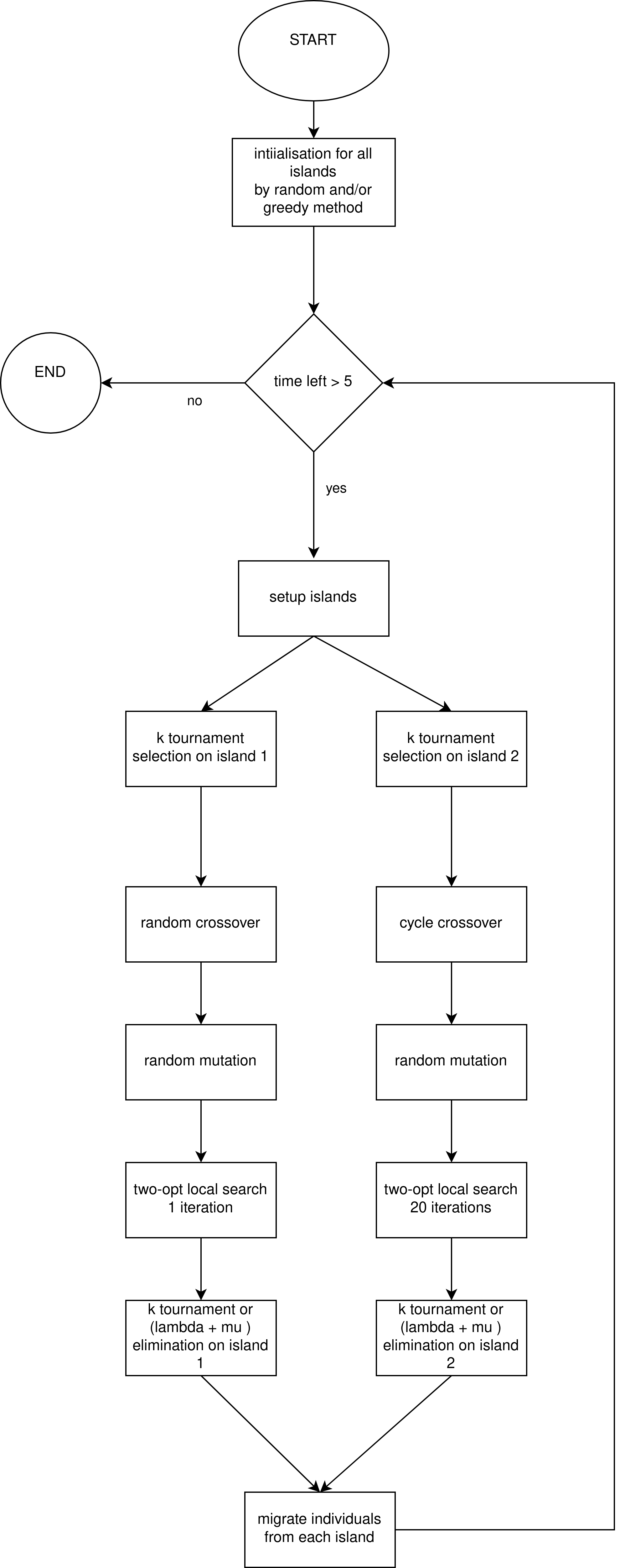
10. The main loop
As can be seen in the following Figure. It represents a flowchart of the overall genetic algorithm.
11. Parameter selection
Since it is impossible to test all the parameter values to find the
global minimum in a reasonable amount of time, the grid search algorithm
was not chosen. Instead, the code performs a hyperparameter search using
the TPE algorithm provided by the hyperopt library to find the best
combination of hyperparameters. The optimisation process was run for one
hour to find optimal hyperparameter values. The algorithm was run on
problem instances 200, 500, 750 and 1000. Those problems can be found
in the repository.
Tuning the hyperparameters across different problem sizes can help identify parameter settings that perform reasonably well across the board. Once done, the parameter values for each problem size was inspected and on the basis of intuition and experience, a selection was made for a general model of parameters.
There was also an attempt made to check if the hyperparameters selected
were not overfitting by testing it on unseen data such as the tsplib95
library. The optimal values of these problems were given and the exact
loss could be calculated.
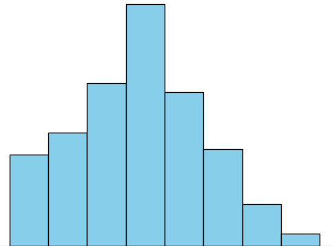
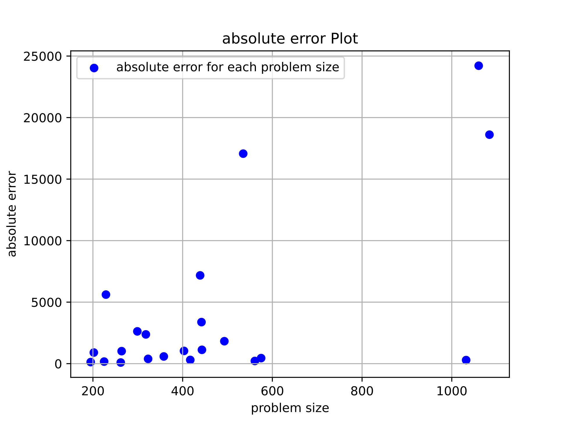
In the appendix, Figure 1 showcases the absolute error for certain problem sizes between 200 and 1100. The absolute errors between 200 and 500 was quite good. Unfortunately, there is quite a big variation in the problem sizes above that, which is understandable since the genetic algorithm also didn’t perform well on those problem sizes when searching for optimal parameter values.
11. Other considerations
-
The island model makes it quite easy for a parallel implementation of the genetic algorithm where each island is run by a separate process using the
multiprocessinglibrary. -
Prepossessing the distance matrix where each
infvalue is replaced by the maximum value of the distance matrix scaled by a factor of 2. -
Another prepossessing step includes computing an adjacency matrix. This is a sorted list of nearest neighbours for each city.
-
Another optimisation is annotating some functions with the help of the
Numbalibrary in order to pre-compile and make the algorithm faster.
12. Numerical experiments
12.1 Metadata
The fixed parameters that were not considered for optimisation include the following:
-
the minimum length of a path to be recombined or mutated, which was set to one third of the path
-
the random initialisation mechanism selects from the top 5 elements, this value was not tested but only selected based on experience.
-
the proportion of random and greedy initialisation was set to 0.9 based on intuition and experience.
-
the amount of individuals to migrate which was 5% of the population of an island was not optimally chosen but selected based on a rule of thumb.
-
the amount of islands in the island model was fixed and set to 2.
As mentioned in the earlier sections, the following parameters were considered for optimisation. The choice of their values can be seen hereunder. The island model requires selecting two values for each variable, resulting in a total selection of 18 parameters.
    lambd   = [30,50]
    alpha   = [0.1, 0.3, 0.5, 0.7, 1]
    beta    = [0.1, 0.3, 0.5, 0.7, 1]
    mu      = [50,100]
    Kselect = [3, 5, 7]
    Kelim   = [3, 5, 7]
    init    = [greedy, random, random & greedy]
    recomb  = [PMX, order_crossover, cycle_crossover, order_backtracking, random]
    local_search_iterations = [1, 5, 20]
The values found by the TPE algorithm for the specific problem
instances are shown in the Appendix. This resulted
in choosing the following parameters for the genetic algorithm. Both islands
do not resemble each other and that is beneficial for the island model.
        config = [{
            "lambdaa":  50,
            "alpha": 0.5,
            "beta": 0.5,
            "mu": 50,
            "Kselect": 3,
            "Kelim": 5,
            "init_method": greedy,
            "recomb_method": random,
            "local_search_iterations": 1,
        },{
            "lambdaa":  50,
            "alpha": 0.1,
            "beta": 0.1,
            "mu": 100,
            "Kselect": 5,
            "Kelim": 7,
            "init_method": random & greedy,
            "recomb_method": cycle_crossover,
            "local_search_iterations": 20,
        }]
The specification of the benchmark machine such as the number of cores, the amount of RAM, and the processor can be seen here:
CPU(s):                  12
Model name:              Intel(R) Core(TM) i7-10750H CPU @ 2.60GHz
Mem:                     15Gi
Python 3.10.12
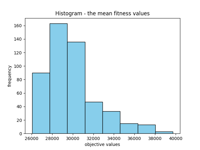
12.2 TSP Tour50
The mean objective value is 34854.030239402106
and the best objective value is 25465.80053443083.
First of all, The algorithm requires on average 8 seconds to report a solution which may seem long, but there is 10 iterations ran between each reporting.
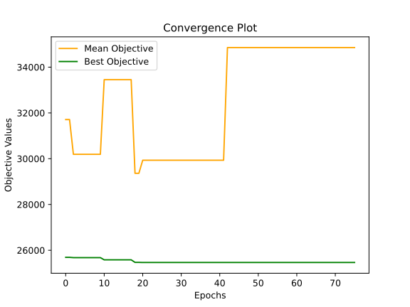
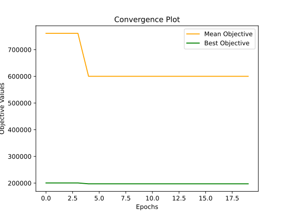
Secondly, with a time limit of 300 seconds, the genetic algorithm utilises the entire allocated time. However, it demonstrates a convergence well before surpassing the specified time constraint, as can be seen in the convergence graph.
Thirdly, The memory usage is also limited. The primary memory allocations are dedicated to storing both the population and offspring, which collectively occupy a relatively small space.
Their total size is calculated as
\((\lambda + \mu) \cdot amount\_of\_cities\)
considering that all entries are integers occupying a minimum of 32 bits
each. A conservative estimate for the lower limit of memory usage can be
calculated as
\((\lambda + \mu) \cdot 50 \cdot 32 = (50 + 50) \cdot 50 \cdot 32 = 20\)
kilobytes.
Additionally, since two islands operate simultaneously, the
combined memory usage increases to at least 40 kilobytes.
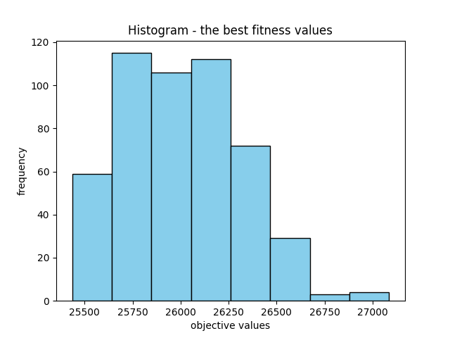
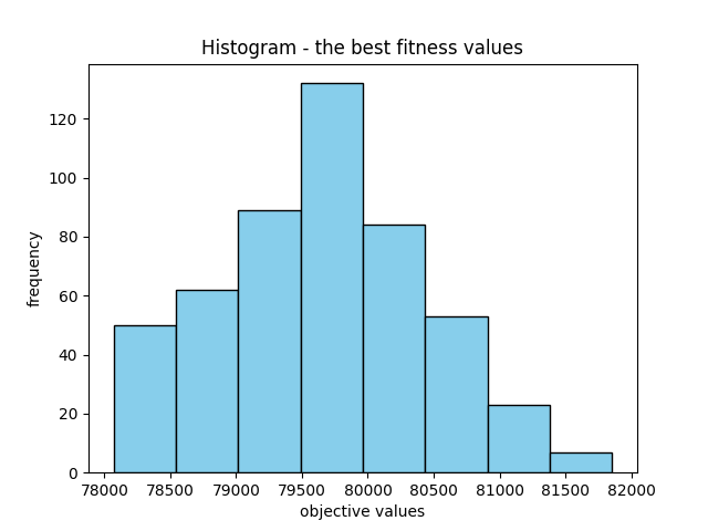
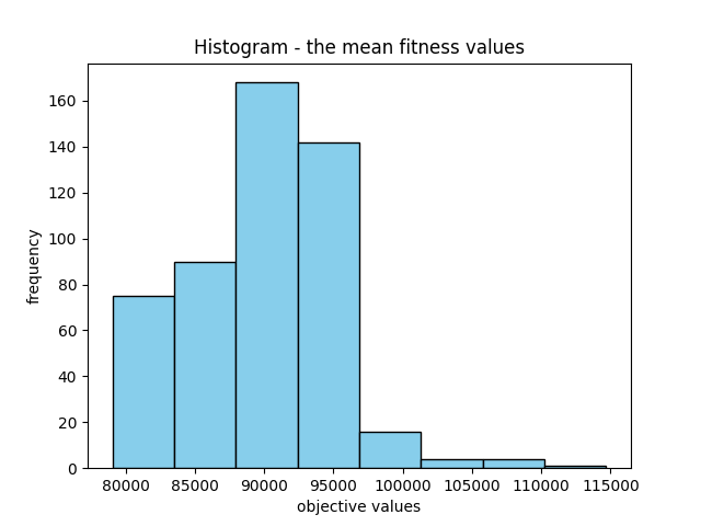
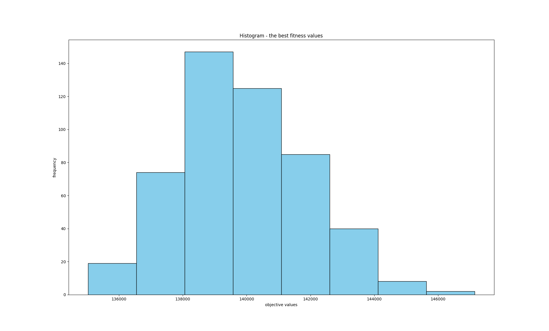
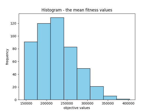
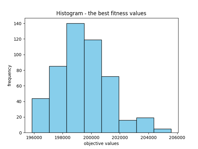
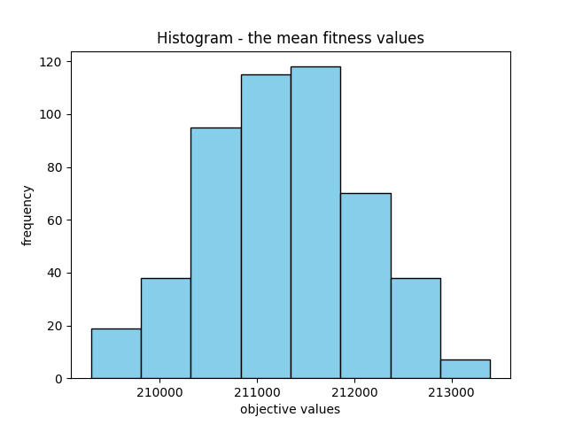
Finally, the mean fitness values display significant variation, which isn’t inherently negative. Instead, it could indicate a diverse set of potential solutions. Conversely, the variance in the best fitness values is relatively lower, which is advantageous. Moreover, it’s beneficial to observe some level of variation in the best fitness values. Absence of such variation might indicate convergence toward a single solution, which is not an ideal scenario.
Standard deviation of mean_values: 2933.2470890444893
Variance of mean_values: 8603938.48538797

Standard deviation of best_values: 430.7019813373877
Variance of best_values: 185504.19672795144
13. Some lessons learned
Genetic algorithms require some expertise to work well in a specific application. Expertise is needed to select the different operators and to determine the correct values for the genetic algorithm parameters. Genetic algorithms also require a lot of tuning and parameter adjustments.
Genetic algorithms are suitable for the problem addressed in this project. This is because genetic algorithms provide an efficient mechanism for exploring the solution space and build on previous successes, allowing them to evolve faster than random algorithms.
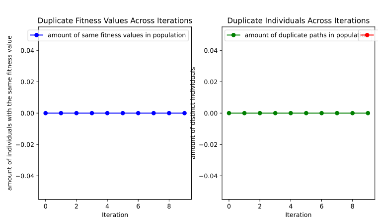
In addition, you need to implement and test certain metrics against the genetic algorithm, which might not be trivial. For instance, determining the number of duplicate solutions or the count of solutions with an infinite cost. Additionally, It could be helpful to measure the computational complexity of the genetic algorithm, such as time per iteration or other relevant metrics and visualise that data. (see both Figure 4 and Figure 3).
14. Future Work
To improve the algorithm, There are a few things that should be
implemented. Firstly, to significantly boost diversification, it’s
necessary to increase the number of islands within the algorithm. Also,
If a population from one island is substantially larger than the
another, it could cause problems during migration. Because, the amount
of solutions to immigrate should be weighted, considering not only the
population size of the source island but also the target island. This is
to not overwhelm the other population too much. This could be avoided by
fixing the amount of individuals to migrate to a constant instead of a
proportion.
Moreover, the addition of various operators is also important in
securing better solutions. It is not enough to have one local search
operator.
Also, the fixed parameters that were set intuitively should rather be
optimally found instead.
References
[1] Introduction to evolutionary computing, Eiben, Agoston E and Smith, James E, 2015, Springer
Appendix
A
B
C
E
# TOUR 200
# [{'lambdaa': 30, 'alpha': 0.5, 'beta': 0.5, 'mu': 100,
'Kselect': 5, 'Kelim': 7, 'init_method': 1, 'recomb_method': 0, 'local_search_iterations': 5},
#  {'lambdaa': 50, 'alpha': 0.5, 'beta': 0.5, 'mu': 50,
'Kselect': 3, 'Kelim': 5, 'init_method': 0, 'recomb_method': 2, 'local_search_iterations': 1}]
# 36372.69542241105

#TOUR 500
# [{'lambdaa': 30, 'alpha': 0.5, 'beta': 0.3, 'mu': 50,
'Kselect': 7, 'Kelim': 5, 'init_method': 0, 'recomb_method': 2, 'local_search_iterations': 1},
#  {'lambdaa': 30, 'alpha': 1,   'beta': 1,   'mu': 100,
'Kselect': 5, 'Kelim': 3, 'init_method': 2, 'recomb_method': 4, 'local_search_iterations': 20}]
# 132369.1570006687

#TOUR 750
# [{'lambdaa': 30, 'alpha': 0.7, 'beta': 0.1, 'mu': 50,
'Kselect': 5, 'Kelim': 7, 'init_method': 2, 'recomb_method': 2, 'local_search_iterations': 5},
#  {'lambdaa': 30, 'alpha': 0.3, 'beta': 0.5, 'mu': 100,
'Kselect': 7, 'Kelim': 5, 'init_method': 2, 'recomb_method': 0, 'local_search_iterations': 1}]
# 197541.09839542626

#TOUR 1000
# [{'lambdaa': 50, 'alpha': 0.5, 'beta': 0.1, 'mu': 50,
'Kselect': 5, 'Kelim': 7, 'init_method': 2, 'recomb_method': 4, 'local_search_iterations': 5},
#  {'lambdaa': 30, 'alpha': 0.1, 'beta': 0.1, 'mu': 100,
'Kselect': 5, 'Kelim': 3, 'init_method': 0, 'recomb_method': 4, 'local_search_iterations': 20}]
# 196618.27939421375
The values for the initialisation methods are encoded as follows:
2:random & greedy, 1:random and 0:greedy.
Also for the recombination methods : 4:random,
3:order_backtracking ,2:cycle_crossover, 1: order_crossover and
0: PMX.
F
tour100
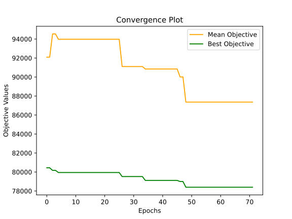
meanObjective, bestObjective, bestSolution
87359.20563684954 78394.94535537285
tour500
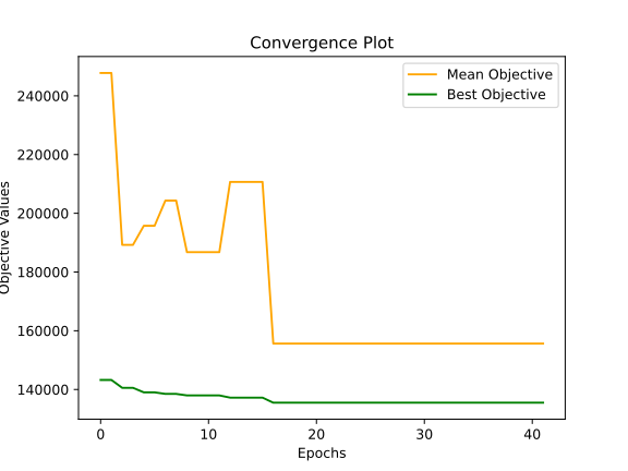
meanObjective, bestObjective, bestSolution
155622.87180627615 135487.1393387503
tour1000
meanObjective, bestObjective, bestSolution
600085.6260011455 197266.16074439613