Solving a Maze with First Order Logic

Author: Ibrahim El Kaddouri

Demonstration:

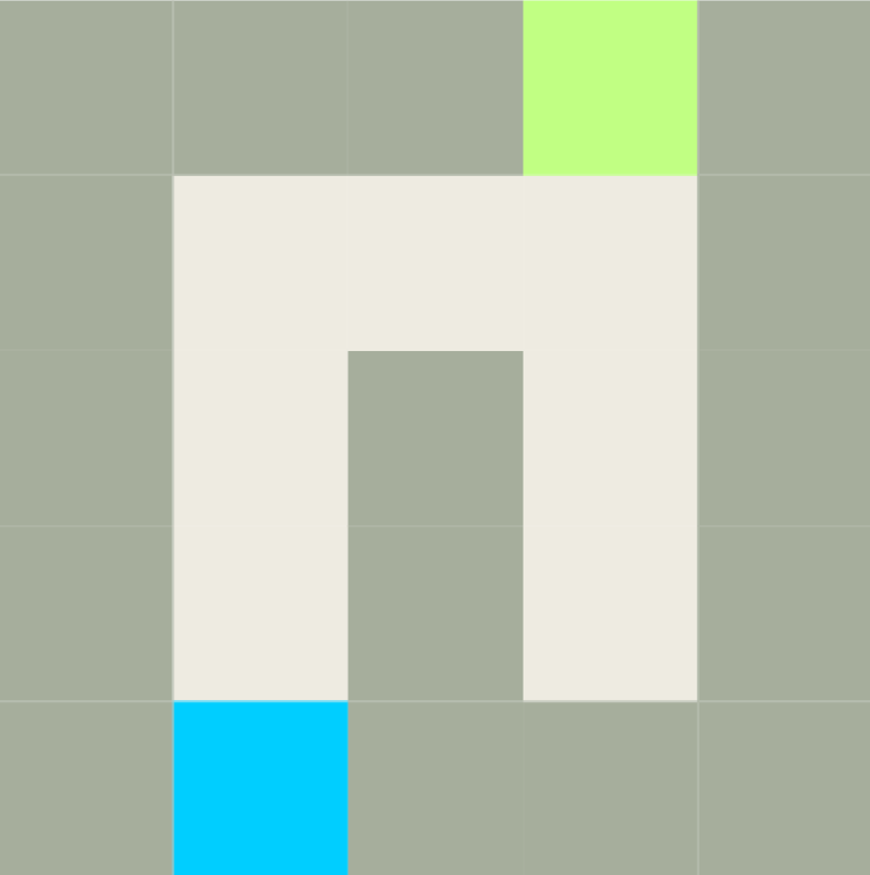
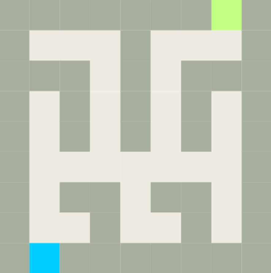
I. Construction Of A Maze

We will write a formal specification of a maze. We will construct a vocabulary in order to use it to write a theory such that only valid mazes are models of the theory.

First, we will clarify some terminology, and introduce the starter vocabulary. We will work in an \(n \times n\) grid made up of cells. There are two top-level type of cells: empty cells and walls. Each empty cell is either a regular empty cell, the entrance, or the exit. Each wall is either an outer wall or an inner wall (although this distinction is merely conceptual, meaning that there is no separate predicate for inner and outer walls in the starter vocabulary). This leads to the following starter vocabulary:

Vocabulary Vstart {
	type X isa nat
	type Y isa nat
	type Pos constructed from {P(X, Y)}
	Wall(Pos)
	Entrance : Pos
	Exit : Pos
}

with the following intended meaning:

X is the set of X coordinates.
Y is the set of Y coordinates.
Pos is a type constructed from X and Y coordinates. The origin is located in the bottom-left corner of the grid. To refer to a cell with coordinates \(X_i\) and \(Y_j\) in our theory, we will use \(P(X_i, Y_j)\). For example, to refer to the bottom-left square, we will use \(P(0, 0)\).
Wall(P(\(X_i, Y_j\))) denotes that a static wall is located at position \(P(X_i, Y_j)\).
Entrance = P(\(X_i, Y_j\)) denotes that the entrance to the maze is located at \(P(Xi, Yj)\).
Exit = P(\(X_i, Y_j\)) denotes that the exit of the maze is located at \(P(X_i, Y_j)\).

The Y coordinates corresponds to rows and X to columns. A valid maze must abide by the following rules.

The position of the start and end cell are fixed. Relative to \(n\), which specifies the size of the maze. the entrance is always positioned in the bottommost row second column. The exit is always positioned in the topmost row, second-to-last column.
All cells in the leftmost and rightmost columns, as well as all cells in the bottommost and topmost rows, are walls, except for the entrance and exit cells which never contain a wall. We will refer to these walls and only these walls as the outer walls. All other walls are inner walls.
From each inner wall, an outer wall can be reached through a connection of neighbouring inner walls (diagonally adjacent cells are not considered neighbours).
Each empty cell can be reached from the entrance through a connection of neighbouring empty cells.
The grid does not contain a 2 × 2 block of walls.
The grid does not contain a 2 × 2 block of empty cells

Here is the full vocabulary and the accompanying theory. You will find in comments more detail about each symbol used.

vocabulary Vmaze {
    extern vocabulary Vstart
    
    neighbor(Pos, Pos)
    inside(Pos)			

    getX(Pos) : X
    getY(Pos) : Y 		

    empty_cell(Pos)
    innerwall(Pos)
    outerwall(Pos)
    
    // these positions are walls and adjacent.
    adjacent_wall(Pos, Pos) 
    
    // these positions are empty cells and adjacent.
    adjacent_empty(Pos, Pos)

    // these positions are walls that are 
    // connected to the outerwall.
    reachable_wall(Pos)
    
    // these positions are empty cells connected
    // to the entrance.
    reachable_empty(Pos) 
}

theory Tmaze : Vmaze {

    // defintion for extraction of x and y components
    {
        ! x[X] y[Y]: getX(P(x, y)) = x.
        ! x[X] y[Y]: getY(P(x, y)) = y.
    }

    // definition for inside cell
    {
        ! p[Pos]: inside(p) <- 
            (getX(p) > MIN[:X]) & 
            (getX(p) < MAX[:X]) & 
            (getY(p) > MIN[:Y]) & 
            (getY(p) < MAX[:Y]). 
    }
    
    // definition for neighbor:
    {
        ! p1[Pos] p2[Pos]: neighbor(p1, p2) <- 
            (getX(p1) = getX(p2)) &
            (getY(p1) = (getY(p2) - 1)).
        ! p1[Pos] p2[Pos]: neighbor(p1, p2) <- 
            (getX(p1) = getX(p2)) & 
            (getY(p1) = (getY(p2) + 1)).
        ! p1[Pos] p2[Pos]: neighbor(p1, p2) <- 
            (getY(p1) = getY(p2)) & 
            (getX(p1) = (getX(p2) - 1)).
        ! p1[Pos] p2[Pos]: neighbor(p1, p2) <- 
            (getY(p1) = getY(p2)) & 
            (getX(p1) = (getX(p2) + 1)).
    }
    
    // defintions for outerwall
    {
        ! p[Pos]: outerwall(p) <- Wall(p) & ~inside(p).
    }
    
    // definition for innerwall
    {
        ! p[Pos]: innerwall(p) <- Wall(p) & inside(p).
    }
    
    // definition for adjacent walls
    {
        ! p1[Pos] p2[Pos]: adjacent_wall(p1, p2) <- 
            (Wall(p1) & Wall(p2)) & neighbor(p1, p2).
    }  
    
    // defintion for reachability from inner to outer
    {
        ! p[Pos]:  reachable_wall(p)  <- outerwall(p).
	! p1[Pos]: reachable_wall(p1) <- ? p2[Pos]: 
            reachable_wall(p2) & 
            adjacent_wall(p1,p2).
    }    
    
    
    // defintion for empty cell
    {
        ! p[Pos]: empty_cell(p) <- ~Wall(p).
    }

    // definition for adjacent_empty
    {
        ! p1[Pos] p2[Pos]: adjacent_empty(p1,p2) <- 
            empty_cell(p1) & 
            empty_cell(p2) & 
            neighbor(p1,p2).
    }    
    
      
    // defintion for reachability of empty cells
    {
        reachable_empty(Entrance).
	    ! p1[Pos]: reachable_empty(p1) <- 
                ? p2[Pos]:  reachable_empty(p2) &    
                            adjacent_empty(p2,p1).
    }
        
            
    // bottom most row are walls
    ! p[Pos]:  (getX(Entrance) ~= getX(p)) &
                getY(p) = getY(Entrance) => Wall(p).
    
    // top most row are walls
    ! p[Pos]:  (getX(Exit) ~= getX(p)) &
                getY(p) = getY(Exit) => Wall(p).

    // left most column are walls
    ! p[Pos]:  getX(p) = MIN[:X] => Wall(p).

    // right most column are walls
    ! p[Pos]:  getX(p) = MAX[:X] => Wall(p).
   
    // the entrance has a fixed position.
    getX(Entrance) = 1.
    getY(Entrance) = 0.
    
    // the exit has a fixed position.
    getX(Exit) = MAX[:X]-1.
    getY(Exit) = MAX[:Y].
    
    // all inner walls must be reachable
    ! p[Pos]: innerwall(p) => reachable_wall(p).
    
    // all empty cells must be reachable
    ! p[Pos]: empty_cell(p) => reachable_empty(p).
    
    // The grid does not contain 
    // a 2 x 2 block of walls.
    ! p[Pos]:   Wall(p) & 
                Wall(P((getX(p)+1), getY(p))) & 
                Wall(P(getX(p), (getY(p)+1))) => 
                empty_cell( P( (getX(p)+1), (getY(p)+1))).
 
    // The grid does not contain 
    // a 2 x 2 block of empty cells.
    ! p[Pos]:   empty_cell(p) & 
                empty_cell(P((getX(p)+1), getY(p))) &
                empty_cell(P(getX(p), (getY(p)+1))) => 
                Wall( P( (getX(p)+1), (getY(p)+1))).
}

structure S : Vmaze {
    X	= { 0..4 }
    Y	= { 0..4 }
    Wall = { 
        P(0, 0); P(4, 4); P(4, 0); P(0, 4); 
                 P(2, 0); P(3, 0); 
        P(0, 1); P(0, 2); P(0, 3);
        P(4, 1); P(4, 2); P(4, 3);
        P(1, 4); P(2, 4);
        P(2,1);  P(2,2);
    }
    Entrance	= P(1,0)   
    Exit	= P(3,4)
      
}

procedure main() {
    model = onemodel(Tmaze, S)
    if model then
    	print(model)
    	initVisualization()
    	visualize(model)
    else
        print("Your theory is unsatisfiable!!!")
    end
}

II. Solving A Maze

We will make a linear time calculus (LTC) theory that models a simple game in which a player-controlled character moves through the maze, in search of the exit. In what follows, we will specify the intended behaviour of this dynamic system, after which we will specify the starter vocabulary.

In the first time point of the game, a player character is positioned at the entrance of the maze, facing upwards. The goal of the game is for the player character to find the exit. The goal is considered completed when the player character has reached the exit. In each time point, the character can move to an empty cell that horizontally or vertically neighbours its current position. The character also has a direction, which is the direction in which the character last moved. For instance, after moving a cell to the right, the character’s direction is to the right.

The tricky part in finding the exit is that the player initially has no idea of what the maze looks like; it is entirely undiscovered! That is: initially, the entire maze – except for the cells horizontally or vertically neighbouring the player character’s starting position – is unknown to the player. As the game proceeds, and the player character moves through the maze, the maze gradually becomes discovered.

Concretely: in each time point, each so far undiscovered cell that horizontally or vertically neighbours the player character, turns from an undiscovered into a discovered cell. This is visualized by the cell turning from a black square into a square that shows the true contents of the cell. After reaching the exit (i.e., once the player character is positioned in the same cell as the exit), the character cannot move anymore. The game can be played through an interactive visualization. The basic behaviour of the game is illustrated using this visualization in the following video.

There is, however, an additional complication to the game: in the search for the exit, the player might encounter a locked gate blocking the way. To unlock a gate, the player must use the appropriate key (while standing in a position that horizontally or vertically neighbours the gate). Keys can be found in the maze and picked up by the player, i.e., by simply being in the same position as the key, the player will possess the key at the next time point.

However, not every key matches every gate. Keys and gates both have numbers. Only the key with the same number as a gate can open that gate. Notice that this information is not displayed in the visualization, this means that you might have to try different keys in the visualization until the right one is selected. When you try to open a gate with a wrong key, there are no effects. If the player uses the appropriate key to open the corresponding gate, both the key and the gate disappear. The player can carry up to three keys at once. The basic behaviour of gates and keys is illustrated in the following video.

In this video, you can see the player character picking up a key (note that the key only goes into the character’s inventory the time point after the character entered the same cell as the key), which is later used to open a gate. Another example, with two gates and two keys, is shown in the following video.

In this video, the player character first picks up a key that does not fit the first gate encountered (i.e., when clicking the key in the inventory, the gate does not open). Later, the player character finds another key that does fit the first gate, and uses it to open that gate.

This leads to the following starter vocabulary:

Vocabulary Vbase {
    type Time isa nat
    Start : Time
    partial Next(Time) isa nat
    
    type X isa nat
    type Y isa nat
    type Pos constructed from { P(X , Y) }
    type Direction constructed from (U , D, L , R)
    
    type Gate isa nat
    type Key isa nat
    Wall(Pos)
    Entrance : Pos
    Exit : Pos
    GateAt(Time, Pos, Gate)
    KeyAt(Time, Pos, Key)
    Discovered(Time, Pos)
    Completed(Time)
    
    PlayerAt(Time) : Pos
    Player Orientation (Time) : Direction
    PlayersKeys(Time, Key)
    
    CanMove(Time , Direction)
    
    I_Gate(Pos, Gate)
    I_Key(Pos, Key)

with the following intended meaning:

Time is a set of time points.
Start is the initial time point.
Next(t) is the successor time point of time point t.
Direction is a type constructed from directions U, D, L and R, respectively denoting up, down, left and right.
Gate is a set of gates, each of which is denoted with a natural number.
Key is a set of keys, each of which is denoted with a natural number.
GateAt(t, p, g) denotes that gate g is positioned at position p at time t.
KeyAt(t, p, g) denotes that key k is positioned at position p at time t. Note that a key’s position is not supposed to move along with the player after the key has been picked up. In other words, a key’s position remains constant for as long as the key has not been picked up. Once a key has been picked up, it should not have a position.
Discovered(t, p) denotes that at time t, position p is a discovered position. Note that this is a fluent, not an action. Once discovered, a cell should remain discovered for the rest of the game. Undiscovered cells get visualized as black squares. Discovered cells get visualized as squares that shows the true contents of the cell.
Completed(t) denotes that the exit has been reached by the player character at time t.
PlayerAt(t) = p denotes that time point t the player character is positioned in the cell with position p.
PlayerOrientation(t) = d denotes that at time point t the player character is facing direction d.
PlayerKeys(t, k) denotes that at time t, the player character is in the possession of key k.
CanMove(t, d) denotes that at time t, the player character can move in direction d, meaning that there is an empty cell neighbouring the player in that direction.
I_Gate(p, g) denotes that in the first time point, gate g is positioned at position p.
I Key(p, k) denotes that in the first time point, key k is positioned at position p.
Move(t, d) denotes that in time point t, the Move action is performed in direction d.
Open(t, k) denotes that in time point t, the open action is performed with key k.

Here is once again the full vocabulary and the accompanying theory. You will find in comments more detail about each symbol used.

LTCvocabulary Vtypes {
    extern vocabulary Vbase

    // symbols that are not temporal (i.e., without time)
    I_Discovered(Pos)
    I_Completed(Pos)
    I_PlayerOrientation : Direction
    I_PlayersKeys(Key) 
    I_CanMove(Direction)
    I_PlayerAt(Pos)

    getX(Pos) : X
    getY(Pos) : Y
    partial getDir(Pos,Pos): Direction
    
    neighbor(Pos, Pos)
    inBounds(Pos)
}

// Vocabulary of Actions
LTCvocabulary Vaction {
    extern vocabulary Vtypes
    
    // Player pergorms moving action in certain directin
    Move(Time, Direction)
    
    // Player tryes to open gate with some key
    Open(Time, Key)
}

// Vocabulary of States
LTCvocabulary V_state {
    extern vocabulary Vtypes
    
    // Environment
    GateAt(Time, Pos, Gate)
    KeyAt(Time, Pos, Key)
    Discovered(Time, Pos)
    Completed(Time)							 
    
    // Player stats
    PlayerAt(Time) : Pos
    PlayerOrientation(Time) : Direction
    PlayersKeys(Time, Key)
    
    // Action permissions
    CanMove(Time, Direction)
}

LTCvocabulary Vtime {
    extern vocabulary V_state

    // symbols that are temporal (i.e., with time)
    C_gateAt(Time, Pos, Gate)
    Cn_gateAt(Time, Pos, Gate)
    
    C_keyAt(Time, Pos, Key)
    Cn_keyAt(Time, Pos, Key)
    
    C_Discovered(Time, Pos)
    Cn_Discovered(Time, Pos)
   
    C_Completed(Time)
    Cn_Completed(Time)
    
    C_PlayerAt(Time, Pos)
    Cn_PlayerAt(Time, Pos)
    
    C_PlayersKeys(Time, Key)
    Cn_PlayersKeys(Time, Key)

    C_PlayerOrientation(Time, Direction)
    Cn_PlayerOrientation(Time, Direction)
    
    Blocked(Time, Pos)
}

LTCvocabulary V {
    extern vocabulary Vaction
	extern vocabulary Vtime
}

// TIME THEORY
theory timeTheo : Vtypes {
    {
        Start = MIN[:Time].
        ! t[Time]: Next(t) = t + 1 <- Time(t + 1).
    }
}

theory T_maze : V {
    //---------------------------------
    //---------------------------------    
    // LTC THEORY FOR GATE_AT FLUENT. 
    //---------------------------------
    //---------------------------------

    {
        ! p[Pos] g[Gate] : GateAt(Start, p, g) <- 
            I_Gate(p, g).
            ! t[Time] p[Pos] g[Gate] : GateAt(Next(t), p, g) <- 
            GateAt(t, p, g) & 
            ~Cn_gateAt(Next(t), p, g).
    }

    {
        ! t[Time] p[Pos] g[Gate] : Cn_gateAt(Next(t), p, g ) <- 
            ?q [Pos] : 	Open(t, g) & 
                        PlayerAt(t) = q &
                        neighbor(p,q).
    }

    //---------------------------------
    //---------------------------------    
    // LTC THEORY FOR KEYAT FLUENT. 
    //---------------------------------
    //---------------------------------

    {
        ! p[Pos] k[Key] : KeyAt(Start, p, k) <- I_Key(p, k).
            ! t[Time] p[Pos] k[Key] : KeyAt(Next(t), p, k) <- 
            KeyAt(t, p, k) & 
            ~Cn_keyAt(Next(t), p, k).
    }

    {
            ! t[Time] p[Pos] k[Key] : Cn_keyAt(Next(t), p, k ) <- 
            ? d[Direction]: PlayerAt(t) = p &
                            Move(t, d).
    }


    //---------------------------------
    //---------------------------------    
    // LTC THEORY FOR DISCOVERED FLUENT. 
    //---------------------------------
    //---------------------------------

    {
        ! p[Pos] : Discovered(Start, p) <- 
            ?q [Pos] : PlayerAt(Start) = q &
                       (neighbor(p,q) | q = p).

        
        ! t[Time] p[Pos] : Discovered(t, p) <-
            C_Discovered(t, p).
            ! t[Time] p[Pos] : Discovered(Next(t), p) <-
            Discovered(t, p) & 
            ~Cn_Discovered(Next(t), p).
    }
       
    {
        ! t[Time] p[Pos] : C_Discovered(Next(t), p) <- 
            ?q [Pos]:   PlayerAt(Next(t)) = q & 
                        (neighbor(p,q) | q = p).
            ! t[Time] p[Pos] : Cn_Discovered(Next(t), p) <- false.
    }
          
    //---------------------------------
    //---------------------------------    
    // LTC THEORY FOR COMPLETED FLUENT. 
    //---------------------------------
    //---------------------------------
     
    {
        Completed(Start) <- false.
        ! t[Time] p[Pos] : Completed(t)	<- 
            C_Completed(t).
            ! t[Time] p[Pos] : Completed(Next(t) <- 
            Completed(t) & 
            ~Cn_Completed(Next(t)).
    }

    {
            ! t[Time] : C_Completed(Next(t)) <-
            PlayerAt(Next(t)) = Exit.
    }


    //---------------------------------
    //---------------------------------    
    // LTC THEORY FOR PLAYERSKEYS FLUENT. 
    //---------------------------------
    //---------------------------------

    {
        ! k[Key] : PlayersKeys(Start, k) <- false.
        ! t[Time] k[Key] : PlayersKeys(t,k) <- 
            C_PlayersKeys(t, k).
            ! t[Time] k[Key] : PlayersKeys(Next(t),k) <-
            PlayersKeys(t,k) & 
            ~Cn_PlayersKeys(Next(t), k).
    }

    {
        ! t[Time] p[Pos] k[Key] : C_PlayersKeys(Next(t), k) <-
            KeyAt(t, p, k) & PlayerAt(t) = p.
        ! t[Time] k[Key] : Cn_PlayersKeys(Next(t), k) <- 
            ?p,q [Pos] : Open(t,k) & 
                         GateAt(t,p,k) & 
                         PlayerAt(t) = q & 
                         neighbor(p,q).
    }

    //---------------------------------s
    //---------------------------------    
    // LTC THEORY FOR CANMOVE FLUENT. 
    //---------------------------------
    //---------------------------------

    {
        ! t[Time] d[Direction] : CanMove(t, d) 	<-
            ?q[Pos] p[Pos]: PlayerAt(t) = q &
                            neighbor(q, p) & 
                            ~Blocked(t,p) & 
                            inBounds(p) &
                            getDir(q,p) = d &
                        q~=Exit. 
    }

    //---------------------------------
    //---------------------------------    
    // LTC THEORY FOR PlayerAt FLUENT. 
    //---------------------------------
    //---------------------------------

    {
        !x[X] y[Y] : PlayerAt(Start) = Entrance.
        !t[Time], p[Pos]: PlayerAt(t) = p <- 
            C_PlayerAt(t, p).
        !t[Time], p[Pos]: PlayerAt(Next(t)) = p <- 
            PlayerAt(t) = p & 
            ~Cn_PlayerAt(Next(t), p).
    }   

    {
        ! t[Time] x[X] y[Y] : C_PlayerAt(Next(t), P(x,y+1))  <-  
            PlayerAt(t) = P(x,y) & Move(t, U). 
        
        ! t[Time] x[X] y[Y] : C_PlayerAt(Next(t), P(x-1,y))  <-  
            PlayerAt(t) = P(x,y) & Move(t, L).
        
        ! t[Time] x[X] y[Y] : C_PlayerAt(Next(t), P(x+1,y))  <-  
            PlayerAt(t) = P(x,y) & Move(t, R).
        
        ! t[Time] x[X] y[Y] : C_PlayerAt(Next(t), P(x,y-1))  <- 
            PlayerAt(t) = P(x,y) & Move(t, D).

        !t[Time], p[Pos], d[Direction] : Cn_PlayerAt(Next(t), p) <-  
            PlayerAt(t) = p & 
            ?q[Pos]: C_PlayerAt(Next(t), q) & 
                     q ~= p.
    }

    //---------------------------------
    //---------------------------------    
    // LTC THEORY FOR PlayerOrientation FLUENT. 
    //---------------------------------
    //---------------------------------

    {
        
        !x[X] y[Y], d[Direction] : PlayerOrientation(Start) = d <-
            CanMove(Start, d).
        !t[Time], d[Direction]: PlayerOrientation(t) = d <-
            C_PlayerOrientation(t, d).
        !t[Time], d[Direction]: PlayerOrientation(Next(t)) = d 	<-
            PlayerOrientation(t) = d & 
            ~Cn_PlayerOrientation(Next(t), d).
    }

    {
        ! t[Time] : C_PlayerOrientation(Next(t), U)  <-  
            Move(t, U). 
        
        ! t[Time] : C_PlayerOrientation(Next(t), L)  <-  
            Move(t, L).
        
            ! t[Time] : C_PlayerOrientation(Next(t), R)  <-  
            Move(t, R).
        
        ! t[Time] : C_PlayerOrientation(Next(t), D)  <- 
            Move(t, D).
        
    }

    //---------------------------------
    //---------------------------------    
    // Action concurrency axioms
    //---------------------------------
    //---------------------------------


    !t [Time] d1,d2[Direction]: Move(t, d1) & 
        Move(t, d2) => d1 = d2.
    !t [Time] k1,k2[Key]: Open(t, k1) &
        Open(t, k2) => k1 = k2.

    //---------------------------------
    //---------------------------------    
    // HELPER FUNCTIONS. 
    //---------------------------------
    //---------------------------------

    // defintion for extraction of x and y components
    {
        ! x[X] y[Y]: getX(P(x, y)) = x.
        ! x[X] y[Y]: getY(P(x, y)) = y.
    }

    // diagonally adjacent cells are not considered neighbours.
    {
        ! p1[Pos] p2[Pos]: neighbor(p1, p2) <- 
            (getX(p1) = getX(p2)) & (getY(p1) = (getY(p2) - 1)).
        ! p1[Pos] p2[Pos]: neighbor(p1, p2) <- 
            (getX(p1) = getX(p2)) & (getY(p1) = (getY(p2) + 1)).
        ! p1[Pos] p2[Pos]: neighbor(p1, p2) <- 
            (getY(p1) = getY(p2)) & (getX(p1) = (getX(p2) - 1)).
        ! p1[Pos] p2[Pos]: neighbor(p1, p2) <- 
            (getY(p1) = getY(p2)) & (getX(p1) = (getX(p2) + 1)).
    }
              
    {
        ! x[X] y[Y] : getDir(P(x,y),P(x,y+1)) = U <- 
            (y+1) =< MAX[:Y] & 
            y >= MIN[:Y] & 
            x >= MIN[:X] & 
            x =< MAX[:X] .
        
        ! x[X] y[Y] : getDir(P(x,y),P(x,y-1)) = D <- 
            (y-1) >= MIN[:Y] & 
            x =< MAX[:X] & 
            x >= MIN[:X] &
            y =< MAX[:Y].
        
        ! x[X] y[Y] : getDir(P(x,y),P(x-1,y)) = L <- 
            (x-1) >= MIN[:X] &
            y =< MAX[:Y] &
            y >= MIN[:Y] &
            x =< MAX[:X].
        
        ! x[X] y[Y] : getDir(P(x,y),P(x+1,y)) = R <- 
            (x+1) =< MAX[:X] &
            y =< MAX[:Y] &
            y >= MIN[:Y] &
            x >= MIN[:X].
    }

    {
       ! x[X] y[Y] : inBounds(P(x,y)) <- 
            y =< MAX[:Y] & 
            y >= MIN[:Y] & 
            x >= MIN[:X] & 
            x =< MAX[:X].
    }

    {
        !t[Time], p [Pos] : Blocked(t, p) <- 
            Wall(p) | ?g[Gate] : GateAt(t,p,g).  
    }   
}

procedure getModel() {
    local St = clone(S);
    setvocabulary(St, V);
    St[V::Time.type] = range(0,5)
    
    local complete_theory = merge(timeTheo, Tmaze)
    model = onemodel(complete_theory, St)
    if model then
        print(model)
    else
        print("Your theory is unsatisfiable!!!")
    end
}