Multi Agent Reinforcment Learning With Dots And Boxes

Authors: Ibrahim El Kaddouri, Staf Rys and John Gao.

1. Introduction

When moving from single-agent RL to multi-agent RL (MAL), game theory plays an important role as it is a theory of interactive decision making.

In this paper, some elementary game theoretic concepts will be used in combination with multi-agent learning, which is non-stationary and reflects a moving target problem (see [1] for basic concepts about game theory when less familiar).

We will start by tackling some canonical games from the ‘pre-Deep Learning’ period. To learn how (multi-agent) reinforcement learning and game theory relate to each other, we will work with tabular RL methods using \(\epsilon\)-greedy and Boltzmann exploration [2][3] and express them using replicator dynamics [4].

Afterwards we move to the Dots-and-Boxes game, first using the minimax algorithm from game-theory [1] and second using RL and machine learning (for some Deep RL references see [5] [6]).

We will be working in the OpenSpiel open-source software framework. OpenSpiel is a collection of environments, algorithms and game-theoretic analysis tools for research in general reinforcement learning and search/planning in games. OpenSpiel supports n-player zero-sum, cooperative and general- sum games [7].

2. Nash & Pareto equilibria

2.1 Game theory in matrix games

The 4 games we will consider, can be categorized in a few different categories: social dilemma games (prisoner’s dilemma), zero-sum games (biased rock paper scissors) or coordination games (subsidy game, battle of the sexes)

2.1.1 Prisoner’s Dilemma

A classic game involving two players, who decide to cooperate C with each other, or defect D from each other, without knowing the other player’s decision. It can be seen from the payoff table that cooperation of both leads to a point of pareto optimality, since none of the agents can improve their result without negatively affecting the other.

	C	D
C	-1, -1	-4, 0
D	0, -4	-3, -3

Meanwhile, if both defect, a Nash equilibrium is reached: given the other agent’s choice to defect, the current agent will always choose to also defect to achieve an optimal result.

2.1.2 Biased Rock Paper Scissors

In biased rock paper scissors, not every match-up has the same result, as seen in the payoff table.

	R	P	S
R	0	-0.25	0.5
P	0.25	0	-0.05
S	-0.5	0.05	0

For example, playing rock against scissors rewards the winning player more than when winning with paper against rock. As a player will not stick to the same option in every situation, there is no pure Nash equilibrium. This results in an optimal mixed strategy of probabilities \(\frac{10}{16}, \frac{5}{16}, \frac{1}{16}\) for playing rock, paper and scissor respectively. This is found by formulating the expected payoffs for each move in terms of their respective probability and value in the payoff table, and then setting the derivative of the expected payoffs to zero. Solving these equations for the probabilities then results in values shown above. Every match-up can be seen as pareto optimal, since there is no situation where one agent can improve their result without affecting the other negatively.

2.1.3 Subsidy Game

In this game, two players, usually companies or central authorities, can choose to perform one of two actions: offering subsidy 1 or subsidy 2, investing in a certain field or another field. As seen in the payoff table, the pareto optimal point is when both players subsidise in the same field: there is no other situation where an agent can improve their result without harming the other.

	S1	S2
S1	-1, -1	1, 1
S2	1, 1	-1, -1

There is also a Nash equilibrium in this point: given the choice of the other agent to subsidise in a field, the current agent wouldn’t want to not subsidise in that same field, since this would reduce their payoff. Remark that two such points exists, because there are two possible ways to reach consensus about the chosen subsidy.

2.1.4 Battle of the Sexes

In this game, called battle of the sexes, a husband and wife wish to go to the movies or the opera: O or M. They much prefer to go together rather than to do different activities, but while the wife prefers O, the husband prefers M. The payoff matrix is can be seen in the following table:

	O	M
O	3, 2	0, 0
M	0, 0	2, 3

This game has two pure strategy Nash equilibria, one where both the husband and the wife choose O, and another where both choose M. In the mixed strategy equilibrium the man chooses M with probability \(\frac{3}{5}\) and the woman chooses O with probability \(\frac{3}{5}\), so they end up together at M with probability \(\frac{6}{25} = \frac{2}{5} \cdot \frac{3}{5}\) and together at O with probability \(\frac{6}{25} = \frac{2}{5} \cdot \frac{3}{5}\). Then the mixed Nash equilibrium is a miscoordination between the man and the woman with a probability of \(\frac{13}{25}\).

3. Learning & Dynamics

3.1 Independent learning in benchmark matrix games

A primitive way to solve the multi-agent problem is to ignore the other agents, essentially transforming it to a single-agent problem, where interactions with the other agents are represented as stochastic noise, this is called independent learning.

The implemented algorithms all utilize tabular Q-learning, differing in their action selection strategies. Further details on this aspect will be provided in Section 3.2.
In Table 1, Nash equilibria are represented using tuples, where the first entry signifies the probability of the first agent selecting the first action, and the second entry represents the probability of the second agent selecting the first action. The same is done for the pareto optima in Table 2.

Nash Equilibrium	ϵ-greedy	Boltzmann	Lenient Boltzmann
(0, 0)	Yes	Yes	Yes

Nash Equilibrium	ϵ-greedy	Boltzmann	Lenient Boltzmann
((0.625 , 0.3125), (0.625 , 0.3125))	No	No	No

Nash Equilibrium	ϵ-greedy	Boltzmann	Lenient Boltzmann
(1, 1)	No	No	Yes
(0, 0)	Yes	Yes	Yes
(0.9,0.9)	Yes	No	No

Nash Equilibrium	ϵ-greedy	Boltzmann	Lenient Boltzmann
(0.6, 0.4)	No	No	No
(1,1)	No	Yes	Yes
(0,0)	Yes	Yes	Yes

For the different benchmark matrix games, the initial actions are as follows. In the prisoner’s dilemma, the initial action is cooperation where \((0, 0)\) indicates \(0\%\) probability of cooperation for the first and second agents. In the biased rock paper scissors game, the actions are ordered as rock, paper, scissors. For instance, \((0.625, 0.3125)\) indicates that the first agent selects Rock with a probability of \(0.625\) and Paper with a probability of \(0.3125\). The probability of the first agent selecting scissors can be derived by subtracting these probabilities from 1. Lastly, in the subsidy game, the first action is S1 and in the battle of the sexes it is opera or O.

Pareto Optimum	ϵ-greedy	Boltzmann	Lenient Boltzmann
(1, 1)	No	No	No

Pareto Optimum	ϵ-greedy	Boltzmann	Lenient Boltzmann
((0.625, 0.3125), (0.625 , 0.3125))	No	No	No

Pareto Optimum	ϵ-greedy	Boltzmann	Lenient Boltzmann
(1, 1)	No	No	Yes

Pareto Optimum	ϵ-greedy	Boltzmann	Lenient Boltzmann
(1,1)	No	Yes	Yes
(0,0)	Yes	Yes	Yes

3.2 Dynamics of learning in benchmark matrix games

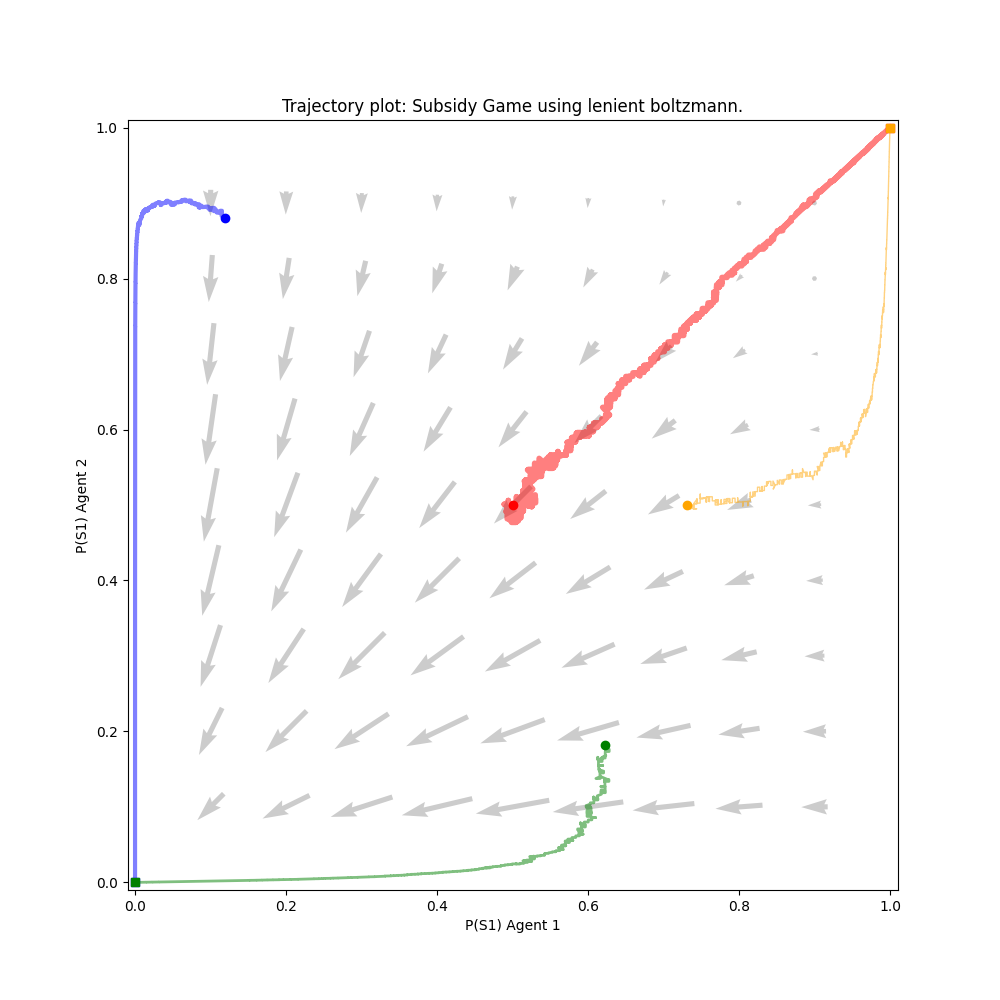
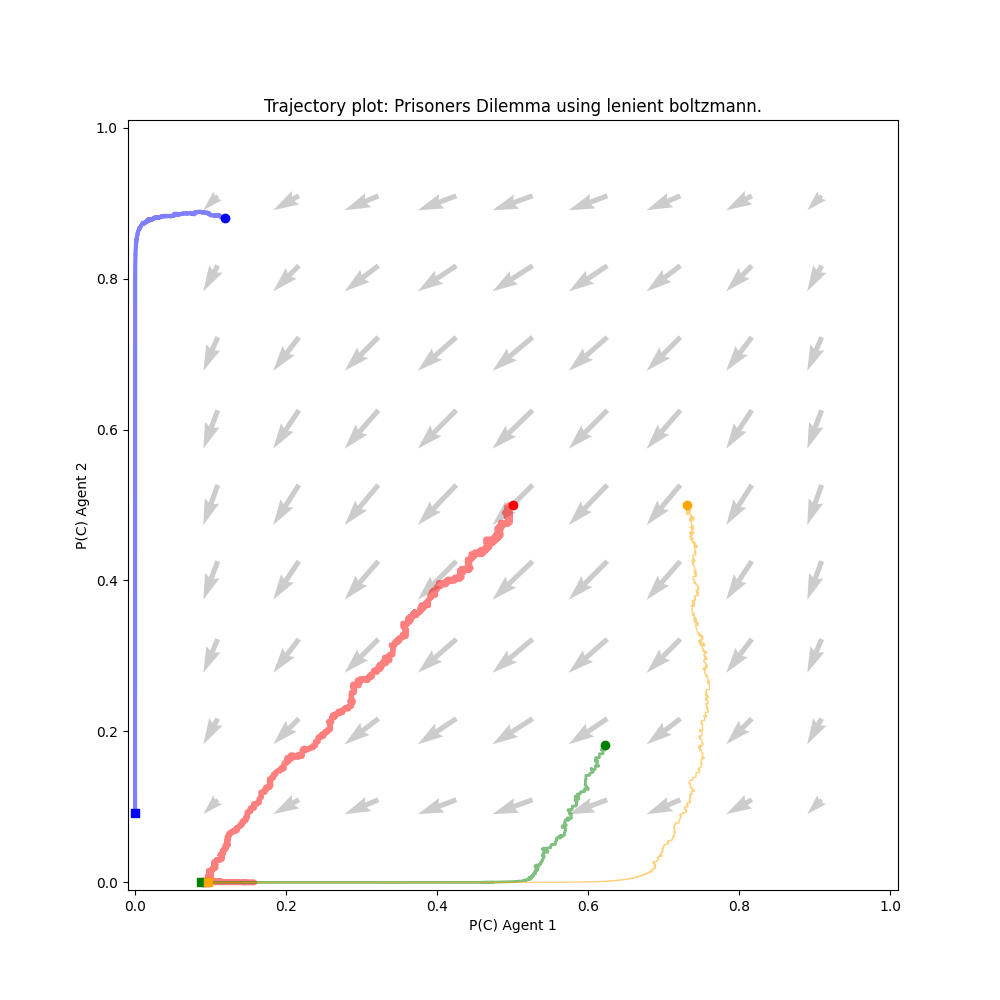
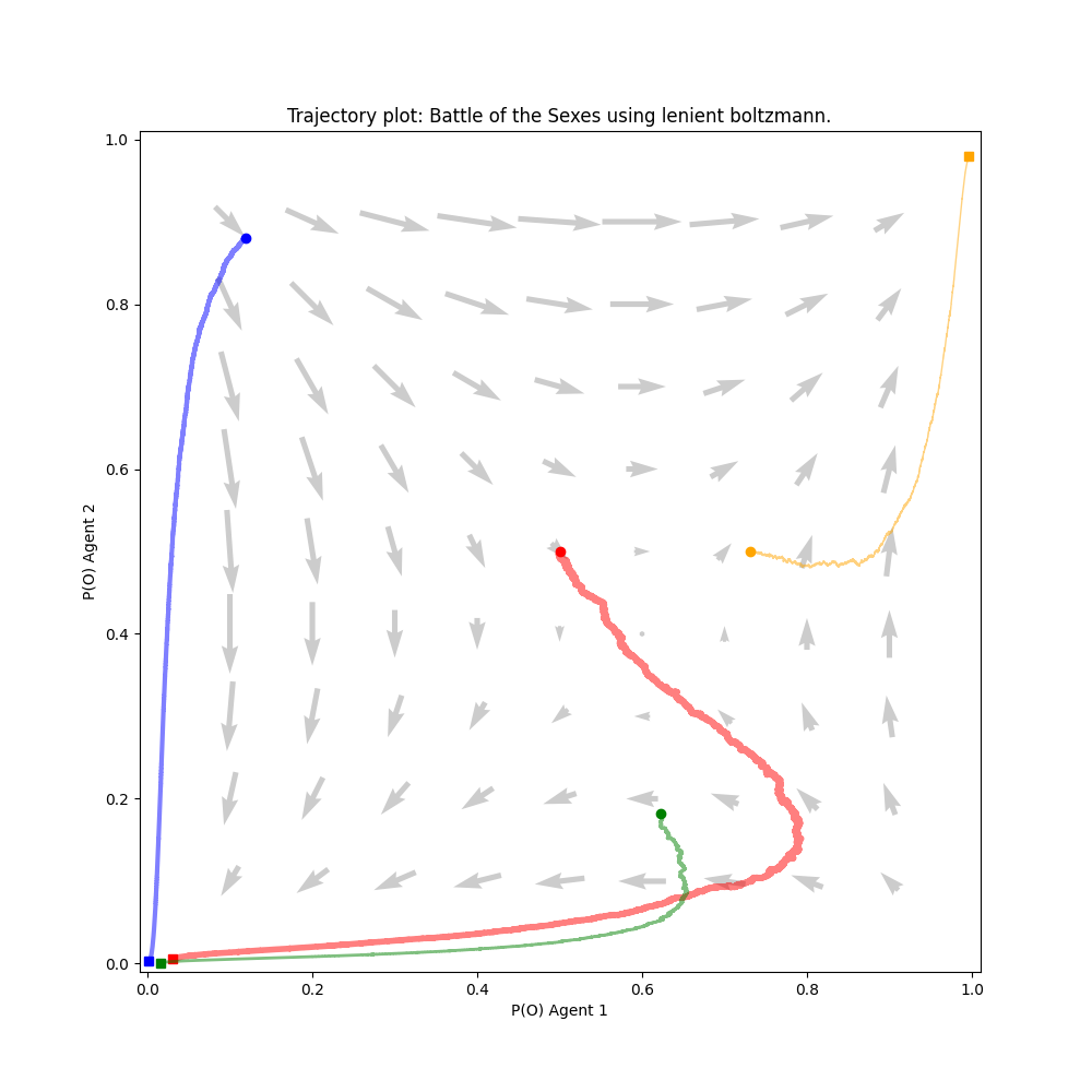
On Figure 1, the directional field and four trajectories for the implemented 2-player lenient Boltzmann agent are plotted. A trajectory starts at a bullet marker and ends at a square marker. The intuition behind the chosen parameter values is explained in paragraph 3.2.1. The endpoints typically converge to Nash equilibria, although there are exceptions such as the game of biased rock paper scissors. Following a trajectory from start to end complies to the directions dictated by the directional field. A notable exception to this tendency are the 2 trajectories converging to (1,1) in the subsidy game. As this point is a pareto optimum, this is not a problem.

The non-complying curvatures at the beginning of the trajectories can be attributed by the overestimation of the Q-values due to leniency. When taking the highest reward of a collection of κ elements, but taking κ steps while doing so results in a delay in updating those values in comparison with regular Boltzmann learning. The concept of leniency will be discussed in further detail in the following section.

3.2.1 Tuning

Two often used action selection mechanisms are ε-greedy and Boltzmann exploration.

ε-greedy

This algorithm selects the best action (w.r.t. Q) with probability 1 − ε, and with probability ε it selects an action at random. Regarding ε, a parameter defined from 0 to 1, three values were chosen evenly spread across this interval. Extremes of this interval are likely to result in poor trajectories, as there would not be an appropriate trade-off between exploration and exploitation during training.

Boltzmann exploration

This mechanism makes use of a temperature parameter τ that controls the balance between exploration and exploitation. A large τ implies that each action has roughly the same probability, while a small τ leads to more greedy behavior. As this parameter is defined from \(0\) to ∞, we first choose the default parameter initialized by the OpenSpiel library. Additionally, we select a parameter value of \(1\), where the softmax function is applied directly on the Q-values. Subsequently, we choose a value that is \(5\) times bigger than \(1\), as \(0.2\) is \(5\) times smaller than 1. After experimentation, it appears that 5 can be seen as an upper limit, as it results in trajectories concentrating around \((0.5, 0.5)\) in the plots. This creates a much more narrow domain of useful values of τ, namely the interval \([0,5]\).

Lenient Boltzmann

The same mechanism as normal Boltzmann but with an additional parameter. The parameter κ determines the amount of rewards that needs to be stored for each action before updating the Q-value based on the highest of those rewards. The following values for each parameter has been experimented upon. As for κ, a parameter defined from 2 to ∞, we consider that a κ value of 1 will result in the traditional Boltzmann tabular learner, while a large value of κ will limit updates to the Q-values. Hence, we chose values of 5 and 10. Upon experimenting, it was clear that the mentioned earlier delay effect on the curve was negatively effecting the dynamics in case of κ = 10. With only 2 actions per agent, there is a \(\frac{1}{4}\) chance of obtaining the highest reward for each action if the other agent chooses its action uniformly. During the training in selfplay, we opted for 100 000 iterations as previous attempts with 1000 and 50 000 iterations didn’t return satisfying dynamics. For τ the tradeoff between exploration and exploitation is achieved by using a linear schedule varying from 0.5 to 0.01, as the exploration can decrease gradually as the dynamics progress with this schedule in favor of a gradual increase in exploitation of the rewards. The step size was set to 0.001 to allow a relatively fast convergence while not losing the details of the learning process due to underfitting.

4 Minimax of small Dots-and-Boxes

In this section we describe how we implemented an optimization of the provided naive minimax template. The impact of using all steps is measured in an experiment.

4.1 Transposition tables

The rationale for choosing the ‘dots and boxes notation’ for representing the board state is based on the paper by Barker and Korf [8].

Dots-and-Boxes is characterized as impartial, meaning that the available moves are solely determined by the board configuration, independent of the current player. Since Dots-And-Boxes is impartial, each state has the same optimal strategy regardless of the current player. This eliminates the need to include the current player in the encoding of our entries. The notation is essentially an enumeration of the states of all edges on the board in a configuration with 1 representing a drawn edge and 0 an edge that is not yet drawn.

For example the notation 1101001... and dimension of the board \(m \cdot n\), the first \((m + 1) \cdot n\) symbols represent the states of the horizontal edges and the last m ⋅ (n + 1) symbols the state of the vertical edges.

The stored values in the transposition table are the calculated minimax value for the configuration encoded in the key. The inclusion of the transposition table only requires minor changes to the naive minimax template. Before performing the recursion step, the current configuration is being looked up in the transposition table, if the configuration is present then a recursion step is avoided and increases the speed of the algorithm. If the configuration isn’t present, then the recursion step is performed and a new entry is added to the transposition table for the configuration.

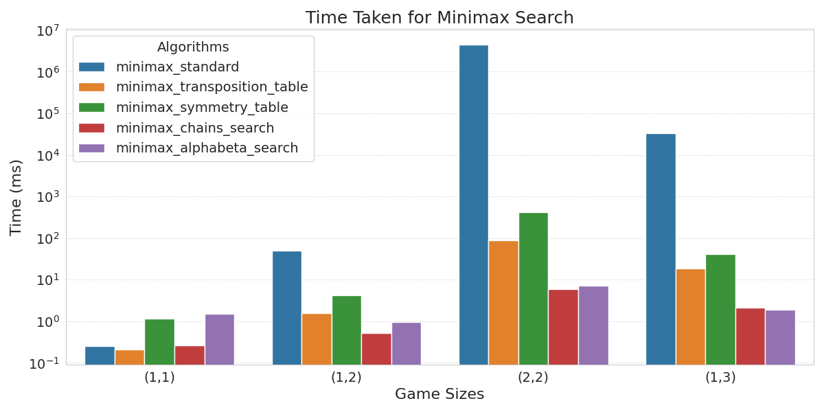
As can be seen in figure 2, this optimization results in a significant decrease in search time compared to standard minimax, as already explored states are taken out of the transposition table when needed and thus don’t need to be reevaluated.

4.2 Symmetries exploitation

As explicitly stated in the paper by Barker and Korf [8]. The mirror image of a state is also a legal game whose optimal strategy mirrors that of the current state. All Dots-And-Boxes instances have horizontal and vertical symmetry, and square boards have diagonal symmetry.

We store canonical representations of states in the transposition table so that all states that are identical under symmetries map to the same entry.
To exploit the symmetries in the game configuration, the current configuration is first looked up in the transposition table. If nothing is found, the horizontal matrix and vertical matrix of the board state are calculated from the Dots and Boxes notation. It is the case that when some transformation is performed on those two matrices, that the resulting board state obtained by combining those two together, is symmetrical to the original board state.

Once these two matrices are calculated, a certain transformation is applied to them, and then the matrices are converted back into the dots and boxes notation. The Dots and Boxes-string for those states can be looked up in the transposition table. If a hit occurs, a recursion step is avoided. When the newly considered configuration is not present in the transposition table, the next transformation in the sequence is calculated and the steps are repeated. When there are no more transformations left then the recursion is executed. The sequence of the calculated transformations is: horizontal mirroring, vertical mirroring, horizontal & vertical mirroring and when the board has a square dimension the rotation of 90 and the rotation of 270 degrees are also part of the sequence.

Figure 2 shows that checking for these symmetries also significantly decreases the search time compared to standard minimax, though it performs a bit worse compared to using a regular transposition table. This is because for every state, all its symmetries are checked, and if unlucky none of them will be in the table. The reason to still check symmetries could be for larger size boards, where this extra cost will become more redundant, as evaluating a state takes a lot more time due to the high branching factor and thus finding one of its symmetries in the table will be very beneficial for the search time.

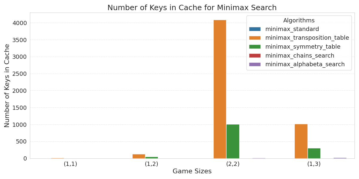
Using symmetries also reduces the space consumption of the table, compared to using a normal transposition table, as can be seen in figure 3. This is because all symmetries of a state are represented as one canonical state in the table.

4.3 Strategies regarding chains

The main ideas for implementing strategies regarding chains were found in the paper [8]. First we give here some additional definitions:

• Half-open chain A chain from which one end is initially capturable (cfr. a dead end street).

• Closed chain A chain from which both ends are initially capturable (cfr. a room)

• Hard-hearted handout A configuration of 2 boxes, capturable with one line.

The first reference describes the optimal moves when chains occur, these strategies can be applied for all chains except for the last one, the player who has to take that turn has to just take all boxes in that last chain:

1. When taking a half-open chain, take all boxes but the last 2 and create a hard-hearted handout.

2. When taking a closed chain, take all boxes but the last 4 and create 2 hard-hearted handouts.

3. When there are multiple chains capturable, take all chains and follow previous rules for the last chain. Closed chains have priority over half-open chains and longer chains have priority over shorter chains.

The reason for the last rule is the difference of 2 in given away boxes between half-open and closed chains of equal length. By following the mentioned rules above, the branching factor of the search tree is significantly reduced, thus speeding up the solving process.

The importance of this technique is that it reduces the number of minimax moves that the algorithm has to consider. Consider a board that has a chain that allows 8 captures in a row. Without the chains technique, minimax has to consider all possible moves that involve partially capturing that chain (e.g. “capture only one box in the chain, then make a non-capturing move”, “capture only two boxes in the chain, then make a non-capturing move”, etc.). The chains technique observes that most of these moves are suboptimal, so minimax can ignore them. Specifically, if a board has a chain with more than two capturable boxes, there are two options that are provably optimal: capture all boxes in the chain (and then make a non-capturing move), or capture all but two boxes in the chain and leave the other two capturable by the opponent. The chain rules are implemented as a subroutine of the minimax algorithm. In particular, the subroutine is used to give back those two provable actions when it recognizes in the board state that there are chains.
Implementing this strategy in minimax results in a significant search time decrease compared to standard minimax, as well as the minimax versions using transposition tables. This is because the search space is heavily reduced, which means that minimax has to evaluate a lot less states.

5 Full Dots-and-Boxes

In the previous task, only small board sizes of Dots-And-Boxes (DAB) were considered and an optimized minimax algorithm was used to solve these boards. Now, for larger board sizes, other algorithms are explored to find more efficient and accurate solutions.

5.1 Evaluation heuristic

In order to use a minimax algorithm in a meaningful way when the board becomes larger, it is necessary to limit the depth of the search. It is not needed to do a complete minimax search of the search graph. In other words, the game is not being solved in its entirety. The search depth is limited to 9 levels, after which a leaf node is reached. The value of this leaf node is then estimated based on the provided configuration of the board. Also, if the leaf node happens to be a terminal node, there will be no need to use any heuristic since the exact score is known. A depth size of 9 is chosen for a specific reason, namely because it is the minimum amount of moves needed in order to find out if a double hard-hearted handout was a good choice.
The value of the heuristic should favor the maximizing player if it is positively large, and should favor the minimizing player if that value is negatively large. In this regard, the amount of boxes captured by the maximizing player and minimizing player are calculated, and then respectively subtracted from each other. In this case, a value of zero means a draw which doesn’t favor any of the two players. A positive value in this node thus favors the maximizing player, while a negative value favors the minimizing player. The larger the absolute value, the more favorable the node is for either the maximizing or minimizing player.

5.2 Alpha-Beta pruning

The decision was made to further improve this minimax algorithm by introducing alpha-beta pruning, a method to reduce the number of nodes in a search tree by pruning irrelevant states, avoiding the need to explore the whole search space . This is especially helpful for larger board sizes of DAB, which have very high branching factors and thus even larger search spaces.
As alpha-beta prunes away unnecessary states, the search space is reduced, meaning minimax has to evaluate less states. Along with the chain strategy, a lot less states need to be evaluated, which means the transposition also contains a lot less keys (figure 3) and the search time decreases (figure 2).

5.3 Important Moves First

When the subroutine developed for the chains technique proposes actions for minimax to explore, it is important to note that there are other moves which take precedence over capturing boxes in chains. Namely actions that result in capturing boxes, but do not cause a chain reaction, i.e. do not cause other boxes to have 3 edges. Those safe capturing moves should be taken first. This reduces the possible actions to only one. Which is an incredible reduction. The same can be said about moves that captures doubletons .

If there are no safe boxes to capture and there are no chains in the board state, the next most important edges are the ones that can be safely captured. Edges are safe to capture if the resulting box will not contain 3 edges. In other words, if there are boxes with less than or equal to one edge already, then another edge can be safely drawn on that box. There could be multiple edges that are safe to draw, but the decision was made to only propose one such edge. This is because in the beginning of the game these are the edges most present and it doesn’t matter much where you place them. This drastically reduces the branching factor in the early stage of the game.

In the case where there are no safe boxes, no chains nor safe edges to capture, we return all possible moves that can be made in the hopes that this list of actions is much smaller and only considered at a later stage in the game, where the number of actions possible is also reduced. Now, for larger board sizes and in order to make an agent that can play on any board size, we must still reduce or limit the number of actions that can be chosen. The number of actions can be limited by randomly shuffling the possible actions and randomly selecting a fixed set of actions or fewer.

5.4 Other Optimization Ideas

Early Termination

There is no need to go further down the recursion tree if the amount of boxes for a particular player is more than half of all the boxes of that game. In that case, we can assume we are in a state of termination and assign the respective rewards.

Move ordering

This following optimization was not implemented due to time limitations, but instead of randomly shuffling the list of actions, we order the list of actions from those that draw an edge at the center of the board first to the edges at the border of the state. Also, actions that would result in the least amount of boxes handed to the opponent should be considered in the order that is beneficial for our agent, i.e. actions that capture the least first. So actions that do not capture any boxes for the opponent are ordered radially from the center after which actions that result in the opponent capturing a box are considered.

Another proposition was to limit the size of the actions that adhere to the long chain rule. This rule goes as follows: Suppose a board with m rows and n columns, if m and n are even, then the first player should aim to make the amount of long chains odd, else he should aim to make the amount of long chains even. In the first iteration of the optimization, a new heuristic function was implemented to give more weight to the moves that obey this rule but due to time constraints, it did not make it to the final agent and our lack of time to optimize it.

5.7 Performance

Against our own agent, the competition was evenly matched, with both agents winning approximately half of the 500 matches. When pitted against a Naive Monte Carlo Tree Search agent, our agent won 431 out of 431 matches. Similarly, in encounters with a randomly acting agent, our agent secured victories in 499 out of 500 matches. Against an opponent utilizing a ‘first open edge’ strategy, our agent won all 500 matches.

opponent	agent wins	opponent wins	timeout
Own Agent	245	255	0
Naive MCTS Agent	431	0	69
Random Agent	499	0	1
First Open Edge Agent	500	0	0

6. AlphaZero

The main idea is that you still use tree search algorithms like minimax or MCTS, but you replace the evaluation function with a neural network. This is the primary difference. Previously, the evaluation function was based on the difference in points scored by both players, but this metric may not always be adequate. For instance, a player could be behind in points yet have much greater control over the board. In the game of dots-and-boxes, this might be because they control long chains, which could be more valuable than points in certain situations.

Another example is that, at the beginning of the game, players typically make random moves due to the game’s nature. However, if we place our lines strategically, we might be able to set up situations later where it is easier to capture chains. As mentioned earlier, controlling long chains is crucial. If we can manage this early on by placing lines strategically, we can significantly improve the model’s performance.

We aim to capture these subtleties using a neural network and train it to recognize favorable board states.

6.1 introduction to AlphaZero

AlphaZero uses a deep neural network \(f_\theta\) with parameters \(\theta\). This neural network takes as an input the board representation \(s\) and outputs both the action probabilities \(p\) and a value \(v\), \((p, v) = f_θ(s)\). The action probabilities \(p\) represents the probability of selecting each action \(a\), \(Pr(a|s)\). The value \(v\) is a scalar evaluation, estimating the probability of the current player winning from position \(s\) [9].

6.2 The NN architecture

For the choice of NN, we have to remember that our agent has to be able to play games of varying board sizes. The agent has to be fast enough to decide each move in less than 200ms.

AlphaZero (AZ) is limited to a fixed board size when it comes to training and playing. This is due to the use of convolutional neural network as the evaluation function in AZ. CNNs are limited to specific input sizes because they process data through a fixed grid structure, like images.

We address this limitation by replacing the CNN with a graph neural network (GNN), a flexible neural network model that can adapt to varying input sizes. This flexibility allows the model to handle multiple board dimensions and even scale up to very large boards without increasing the number of parameters, making it more versatile for different game configurations [10].

More specifics about the exact layers and architecture will be provided the future (sorry). In the meantime, feel free to explore and play the game developed from Chapter 5 at this link.

6.3 representation of dots-and-boxes in GNN

COMING LATER

6.4 training pipeline

COMING LATER

References

[1] Yoav Shoham and Kevin Leyton-Brown. Multiagent systems: Algorithmic, game-theoretic, and logical foundations. Cambridge University Press, 2008.

[2] Karl Tuyls and Gerhard Weiss. Multiagent learning: Basics, challenges, and prospects. Ai Magazine, 33:41–52, 12 2012.

[3] Lucian Busoniu, Robert Babuska, and Bart De Schutter. “A Comprehensive Survey of Multiagent Reinforcement Learning”. In: IEEE Trans. Systems, Man, and Cybernetics, Part C 38.2 (2008).

[4] Daan Bloembergen et al. “Evolutionary Dynamics of Multi-Agent Learning: A Survey”. In: J. Artif. Intell. Res. (JAIR) 53 (2015), pp. 659–697

[5] Yann LeCun, Yoshua Bengio, and Geoffrey E. Hinton. “Deep learning”. In: Nature 521.7553 (2015), pp. 436–444.

[6] Ian J. Goodfellow, Yoshua Bengio, and Aaron C. Courville. Deep Learning. Adaptive computation and machine learning. MIT Press, 2016.

[7] Marc Lanctot et al. “OpenSpiel: A Framework for Reinforcement Learning in Games”. In: ArXiv abs/1908.09453 (2019).

[8] Joseph Kelly Barker and Richard E. Korf. Solving dots-and-boxes. In AAAI Conference on Artificial Intelligence, 2012

[9] Silver, D., Schrittwieser, J., Simonyan, K. et al. Mastering the game of Go without human knowledge. Nature 550, 354–359 (2017). https://doi.org/10.1038/nature24270

[10] Ran El-Yaniv Shai Ben-Assayag. Train on small, play the large: Scaling up board games with alphazero and gnn. 2021.