Author: Ibrahim El Kaddouri, Quentin St-Pierre, Enrico Tonon, Enrique Dorado Gil
Introduction
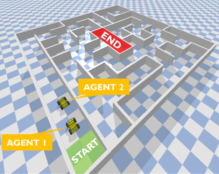
The micromouse competition involves building a small, wheeled robot that autonomously navigates a maze to find the fastest route to the goal. Participants have a maximum of 10 minutes to explore the environment, after which the micromouse attempts to reach the target cell as quickly as possible, with scoring based on the fastest completion time.
In this project, we assume the robot has prior knowledge of the maze, having explored and mapped it, enabling the robot to draw an optimal path from the starting cell to the goal. However, this project diverges significantly from traditional micromouse competitions. Traditional competitions have specific constraints: the maze floor is wooden, the room is well-lit, and there is no significant inclination/tilt of the floor or walls respectively.
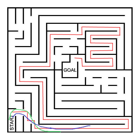
In this project, these constraints are removed. The robot must navigate the maze under various conditions: unknown floor materials (e.g., asphalt, wood, plastic, gravel), outdoor settings with variable lighting and weather conditions (including rain and wind), and changes in elevation. The maze can have an organic shape, with non-constant distances between walls, smooth and sharp turns, and varying corridor widths.
This problem is akin to autonomous racing. Developing an autonomous racing car for circuits can be adapted to solve the micromouse problem. This report focuses on the optimal trajectory for the robot given a specific path. The optimal trajectory is defined as the driving line that allows the robot to take turns as fast as possible while increasing speed without losing control. The robot’s trajectory is defined by position coordinates and a velocity vector: (x(t), y(t), v(t))
Various approaches can achieve the optimal trajectory. One method is to track the path’s centerline closely (which is the shortest path). Another is to calculate the optimal trajectory upfront and let the robot follow it. This report opts for a solution where the robot plans its trajectory itself and controls the vehicle to travel as fast as possible without hitting walls.
Problem Design
Classical Approach
From control theory, advanced models like Model Predictive Control (MPC) can calculate the trajectory, requiring exact knowledge of the vehicle dynamics state. Crucial factors include tire-road contact friction, which changes with aerodynamics, road conditions, weather, and vehicle manoeuvres. The high degree of model uncertainty due to external influences combined with nonlinear effects in tire and vehicle dynamics poses a challenge for algorithms like MPC.
Available models approximate vehicle dynamics to a degree but are computationally demanding, especially with tire models. Current research efforts aim to calculate vehicle dynamics using artificial neural networks, which are computationally faster than classical physical models.
Data Driven Approach
The choice of a data-driven approach (DDA) over a classical algorithmic approach is due to the complexity of modelling the problem’s dynamics. DDA is suitable for problems that are difficult to model or have complex dynamics. Reinforcement learning (RL) is used for planning and control, allowing the robot to learn its trajectory from sensor inputs. Unlike supervised learning, RL enables the robot to discover its optimal behaviour through experience, potentially finding superior trajectories.
In this project, the micromouse is seen as an agent interacting with its environment continuously. At each timestep \(t\), the agent performs an action \(a_t\) that leads to a reward \(r_t\) and observations of the environment state \(s_t\). Based on the reward \(r_t\), the agent maximises the sum of rewards over time, learning specific behaviours in the environment.
Abstraction
Simulation and the Sim-to-Real Gap
Real-life experiments are costly in time and resources. Long-term training can degrade hardware, affecting DRL performance. The robot might need human supervision or even intervention to reset the episode/task. The robot itself cannot run faster than real-time. Simulation is an attractive alternative for data acquisition and task learning, addressing challenges like sample inefficiency. Simulation environments increase available training data and reduce the time and resources needed for real-world interaction.
The micromouse will be simulated in the Pybullet Physics engine, modelled as a double-track or full-vehicle model. The more complex the vehicle dynamics model, the more parameters are needed for the DDA method. However, a significant challenge in simulation-based training is the sim-to-real gap, the mismatch between data collected in simulated environments and real-world settings.
Closing the Sim-to-Real Gap
The sim-to-real gap causes RL algorithms trained on synthetic data to perform worse in real-world settings. Factors contributing to this gap include differences in sensing, actuation, physics, and novel real-world experiences. To ensure DRL trained in simulation works well in real-world applications, the sim-to-real gap must be narrowed through domain randomisation, sensor noise handling, and environment randomness.
Domain Randomization
Domain randomisation uses random parameters in the simulator to account for real-world variability, reducing reliance on biases in training data. For example, instead of precisely modelling friction, random friction coefficients within plausible intervals are used. This approach makes the agent more resilient to real-world mismatches.
Sensor Noise
Sensor noise can be reduced with improved hardware, but it cannot be completely eliminated. The perception subsystem must be designed to be robust against noise, ensuring reliable performance.
Environment Randomness
Real-world environments have both regularity and randomness. For example, while seasons are regular, weather is random. Clear weather is ideal for sensor detection, but changes in weather introduce randomness. Sensor fusion helps cope with environmental randomness, providing reliable detection and localisation.
Sensors and Uncertainties
The micromouse requires both accurate map content and vehicle localisation relative to the map. Vehicle self-localisation can be based on fused sensor information, though this is challenging due to sensor accuracy and accumulated drift. Sensor uncertainties or inaccuracies exist, and high-speed localisation and state estimation are crucial for precise trajectory planning and control.
Dynamic Uncertainties
External disturbances like track banking can be deduced from IMU data with careful post-processing. Track irregularities impact high-frequency suspension and chassis responses. Tire parameters, vehicle mass, and inertia are influential on overall vehicle dynamics, with actuator response being sufficiently measurable. Simulation of dynamic uncertainties, such as tire track contact response, steering rack backlash, and data transport latency’s, is complex. Imperfect actuator calibration adds slight steering offsets, mimicking real-world conditions.
Learning task
The features used for the reinforcement learner varies from paper to paper, but there are some common patterns as follows:
-
linear velocity vector
-
linear acceleration
-
heading angle
-
distance to wall
-
distance to centerline
-
turning rate
-
curvature measurements in the form of a series of discrete points of the sides and middle of the course ahead.
The input normalisation is important in most learning algorithms since different features might have totally different scales.
The control actions are usually the steering angle δ and a throttle or brake request (acceleration) that are sent to low-level controllers for actuating the motor and the brakes.
Given the continuous state and action space, neural networks have been employed as global, non-linear function approximators. There is also the choice of learner to use, it seems that the most common approach include one of the following learners : PPO, A3C, SAC.
Another challenge will be that the actions that the learner infers can result in an unstable driving line of the robot. Therefore it may be helpful to have a PID controller post-process the result of the learner.
Experiments & performance evaluation
To evaluate the performance of the learning agents, several evaluation races are conducted in a simulated test environment (5). In these experiments, the speed and reliability of the trained agent will be monitored and a comparison with the algorithmic approach will be made.
As the objective is to go from start to goal as fast as possible, the evaluation metric will be time. To have a reliable representation of the abilities of the learner, there will be multiple evaluation runs. The difference in time between the learning agent and the algorithmic micromouse could then be plotted to visualise and compare the performance.
Technical challenges
In order to effectively evaluate the performances of the micromouse, the following three aspects are of crucial importance: The reward shaping problem and definition of terminal spaces.
The reward shaping problem
The reward signal is needed in order to communicate to the robot what you want it to achieve, not how. There is not one way of designing the reward system. The most common approach to shape the behaviour of the autonomous robot includes the following elements.
The primary desired behaviour that must be communicated to the agent is not to crash but complete laps of the race track. This behaviour is encoded in an equation called the standard reward, as a positive reward for completing a lap \(r_{complete}\) and punishment for crashing \(r_{crash}\) written as,
\[r_{standard} = \begin{cases} -1 & \text{if crash} \\ 1 & \text{if path complete} \\ \end{cases}\]Due to the sparsity of the standard reward, shaped intermediate rewards are used to aid the learning process. The second reward considered is related to the progress the vehicle has made along the track. The progress reward uses the progress made by the vehicle along the track centerline at each timestep. The difference in progress between the current and previous timesteps is scaled according to the track length and used as a reward. The equation is given down below and the figure illustrates this.
\[r_{progress} = \beta \frac{ (p_{t+1} - p_t)}{L_{track}} \label{eq: progress}\]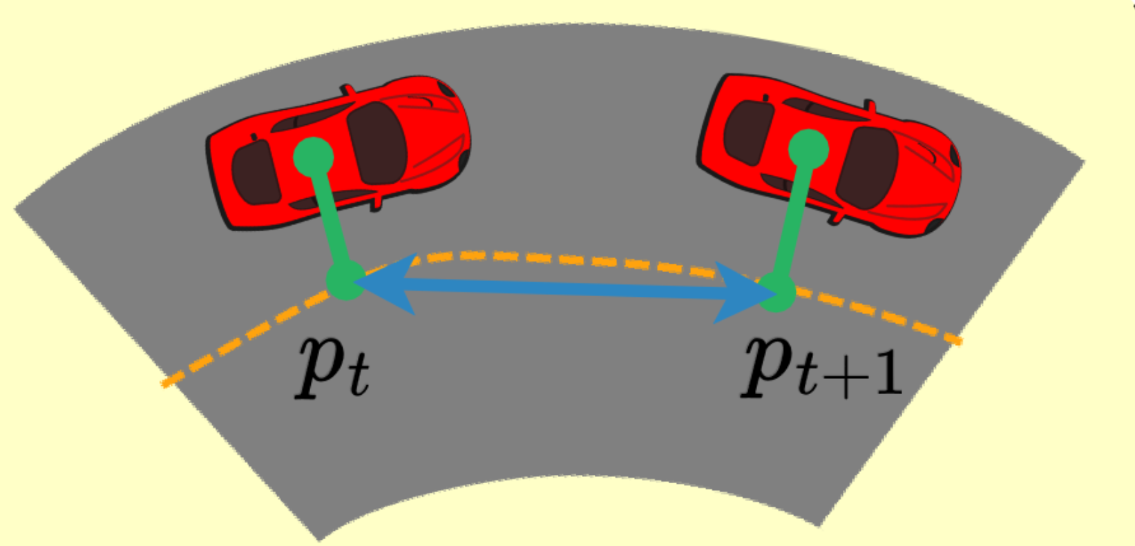
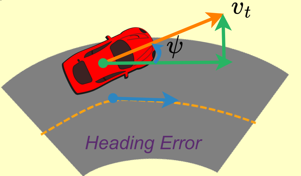
The third reward that is considered uses the vehicle’s velocity in the direction of the track. The velocity along the line is calculated according to the cosine of the difference in angle between the vehicle and the track centerline as shown in the following figure. The heading reward is written as, \(r_h = \frac{v_t}{v_{max}} \cos \psi\)
where \(v_t\) is the speed of the vehicle, \(\psi\) is the heading error.
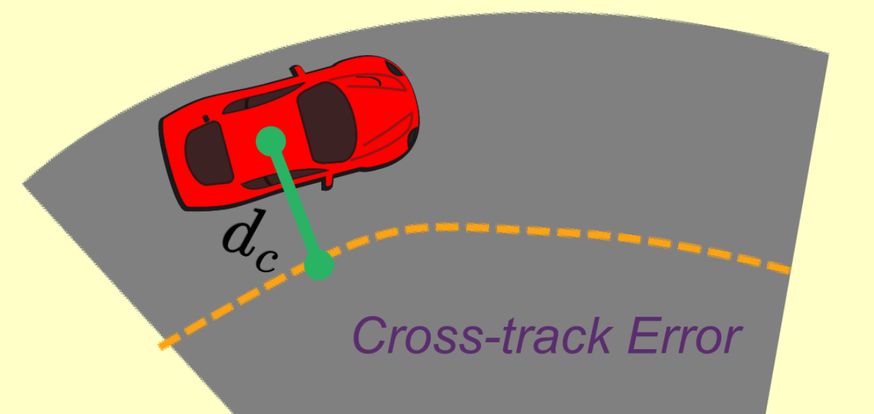
The third reward is an out of bounds punishment. As explained earlier, the micromouse has prior knowledge about the chosen path along the maze that it must follow. To ensure that the micromouse learns to take turns along the right path, negative rewards will be introduced when the micromouse is found to be too far away from the chosen path. More specifically, negative rewards will be given when the distance between the micromouse and the centerline of that chosen path is about the length of the width of the corridors of the maze. In that way, when the micromouse takes the wrong path, he will be penalised and thus it will highly discourage the learner to deviate from the chosen path.
Some considerations for other types of rewards is the following:
-
punishment for driving too slowly
-
penalise duration of the lap
Defining terminal states
There is also subjectivity in defining the criteria for a terminal state. Obviously the finish line of the end cell of the maze does define a terminal state. The following scenario’s are doubtful cases:
-
When crashed to the wall
-
Vehicle is out of bounds (i.e. the robot took a wrong turn in the maze)
-
A maximal time has exceeded