Author: Ibrahim El Kaddouri
Repository:
 The repository is private
Notebook:

5. Adverserial Attacks
5.1 Theory and Implementation
5.1.1 Introduction
This section of the notebook presents an overview on adversarial examples in neural networks, exploring both the theoretical foundations and practical implementations of various attack methods. Adversarial examples are inputs crafted by adding small, carefully designed perturbations to legitimate samples, causing machine learning models to misclassify them. We will explore different attack methods including:
- Fast Gradient Sign Method (FGSM)
- Basic Iterative Method (BIM)
- Projected Gradient Descent (PGD)
- Carlini & Wagner (C&W) Attack
- Generative Adversarial Perturbations (GAP)
By the end of this chapter, you’ll understand how these attacks work, their mathematical foundations, and how to implement and evaluate them against neural network models.
Utils
Before we delve into the problem of developping adverserial attakcs, we will first define some utility function that will help us later down the road. These utility functions do the following:
- Load and preprocess image data from TensorFlow Datasets (TFDS).
- Build simple neural network architectures (MLP and CNN) in TensorFlow/Keras.
- Train and save models, or load existing ones from disk.
- Compute common loss functions for classification tasks.
Each code section includes detailed documentation.
Model Structures
The following are the model architectures that we will be using for testing the robustness of different adverserial attacks.
-
CNN Architecture:
- Two convolutional layers with ReLU activation
- One max pooling layer
- Flattening layer
- Fully connected output layer with softmax activation
-
MLP Architecture:
- Flattening layer to convert 2D images to 1D vectors
- Single hidden layer with 128 neurons and ReLU activation
- Fully connected output layer with softmax activation
def build_mlp(config: ModelConfig) -> tf.keras.Model:
    """
    Build and compile a simple multilayer perceptron (MLP).

    Args:
        config (ModelConfig): Specifies input shape, number of classes, hidden layers, and loss.

    Returns:
        tf.keras.Model: Compiled Keras model.
    """
    assert config.layers is not None, "Dense config must specify 'layers'"
    assert config.loss   is not None

    model = tf.keras.Sequential([
        tf.keras.layers.Input(config.input_shape),
        tf.keras.layers.Flatten(),
        *[tf.keras.layers.Dense(units, activation='relu') for units in config.layers],
        tf.keras.layers.Dense(config.n_classes)
    ], name=config.name)

    model.compile(optimizer=OPTIMIZER,
                  loss=config.loss,
                  metrics=METRICS)
    return model


def build_cnn(config: ModelConfig) -> tf.keras.Model:
    """
    Build and compile a small convolutional neural network (CNN).

    Architecture:
      - Conv2D(32,3) + ReLU
      - Conv2D(64,3) + ReLU
      - MaxPooling2D(2x2)
      - Dropout(0.25)
      - Flatten
      - Dense(128) + ReLU
      - Dropout(0.5)
      - Dense(n_classes)

    Args:
        config (ModelConfig): Specifies input shape, number of classes, and loss.

    Returns:
        tf.keras.Model: Compiled Keras model.
    """
    assert config.loss   is not None
    model = tf.keras.Sequential([
        tf.keras.layers.Input(config.input_shape),
        tf.keras.layers.Conv2D(32, 3, activation='relu'),
        tf.keras.layers.Conv2D(64, 3, activation='relu'),
        tf.keras.layers.MaxPooling2D(2),
        tf.keras.layers.Dropout(0.25),
        tf.keras.layers.Flatten(),
        tf.keras.layers.Dense(128, activation='relu'),
        tf.keras.layers.Dropout(0.5),
        tf.keras.layers.Dense(config.n_classes)
    ], name=config.name)

    model.compile(optimizer=OPTIMIZER,
                  loss=config.loss,
                  metrics=METRICS)
    return model

print("Model builders ready")
5.2 Theoretical Background
The Discovery of Adversarial Examples
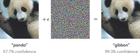
Szegedy et al. (2014) made a remarkable discovery: even state-of-the-art neural networks are vulnerable to adversarial examples. These are inputs that have been subtly modified to cause misclassification, yet remain perceptually identical to the original samples to human observers.
Initially, the cause of adversarial examples was mysterious. However, Goodfellow et al. (2015) demonstrated that linear behavior in high- dimensional spaces is sufficient to cause adversarial examples, challenging the prevailing assumption that the nonlinearity of neural networks was to blame.
Formal Definition of Adversarial Examples
The adversarial example problem can be formally defined as follows: Consider a machine learning system M and an input sample C (called a clean example). Assuming that sample C is correctly classified by the machine learning system, i.e., M(C) = y_true, it is possible to construct an adversarial example A that is perceptually indistinguishable from C but is classified incorrectly, i.e., M(A) ≠ y_true.
A critical observation from Szegedy et al. (2014) was that these adversarial examples are misclassified far more often than examples perturbed by random noise, even when the magnitude of the noise is much larger than the magnitude of the adversarial perturbation.
Categories of Adversarial Attacks
Adversarial attacks can be categorized based on various criteria:
Based on Attack Scenarios:
-
White-box Attacks: The attacker has complete access to the internal model information, including model architecture, weights, and training data. This scenario provides fewer constraints, making it easier to achieve effective attacks.
-
Black-box Attacks: The attacker has limited or no knowledge of the model’s internal structure and can only observe the outputs for given inputs. These attacks are more challenging but more realistic in practical scenarios.
Based on Attack Objectives:
-
Non-targeted Attacks: The goal is simply to cause the model to misclassify the input (changing the prediction to any incorrect class).
-
Targeted Attacks: The adversarial example must be classified as a specific predetermined class. This is considerably more challenging than non-targeted attacks.
We will focus on non-targeted white-box attacks in this article.
Why Linear Models Are Vulnerable
Consider a classifier operating on feature vectors with limited precision. Intuitively, we would expect that if we perturb an input \(x\) by a small vector \(\eta\) where each element is smaller than the precision of the features, the classifier should assign the same class to both \(x\) and \(\tilde{x} = x + \eta\). Formally, for problems with well-separated classes, we expect the same classification when \(|\eta|_\infty < \epsilon\), where \(\epsilon\) is sufficiently small. Now, consider the dot product between a weight vector \(w\) and an adversarial example \(\tilde{x}\):
\[w^\top \tilde{x} = w^\top x + w^\top \eta\]The adversarial perturbation causes the activation to grow by \(w^\top \eta\). To maximize this increase subject to the max norm constraint on \(\eta\), we can set \(\eta = \text{sign}(w)\). This leads to a critical insight: While \(|\eta|_\infty\) does not grow with the dimensionality of the problem, the change in activation caused by perturbation can grow linearly with \(n\). Therefore, in high-dimensional problems, many infinitesimal changes to the input can accumulate to produce one large change in the output.
This explanation shows that even a simple linear model can have adversarial examples if its input has sufficient dimensionality. This is exactly what we will be trying to prove in the following section.
5.3. Adversarial Iterative Attack Methods
The following sections describe different methods to generate adversarial examples, which we will implement and compare.
The following functions implement common adversarial attacks on image classifiers.
Each receives a batch of images and labels, plus an AttackConfig describing
the victim model, perturbation size, steps, and normalization functions.
A. Fast Gradient Sign Method (FGSM)
The Fast Gradient Sign Method (FGSM), introduced by Goodfellow et al. (2014), is a classic white-box attack method. It’s called “fast” because it require only one iteration to compute adversarial examples, making it much quicker than other methods.
FGSM linearizes the cost function around the current parameter values and obtains an \(L_\infty\) constraint constrained perturbation:
\[\eta = \text{sign}(\nabla_x J(\theta, x, y))\]The adversarial example is then generated by:
\[X_{\text{adv}} = X + \epsilon \cdot \text{sign}(\nabla_X J(X, y_{\text{true}}))\]where \(\epsilon\) is a hyperparameter that controls the magnitude of the perturbation.
def fgsm_attack(x_batch: tf.Tensor,
                y_batch: tf.Tensor,
                config: AttackConfig) -> tf.Tensor:
    """
    Fast Gradient Sign Method (FGSM).

    FGSM perturbs each input pixel in the direction that maximally increases loss,
    scaled by epsilon. It requires only one backward pass per batch.

    Args:
        x_batch (tf.Tensor): Batch of normalized images (shape B x H x W x C).
        y_batch (tf.Tensor): True labels (shape B).
        config (AttackConfig): Must contain:
            - epsilon: max perturbation per pixel (float).
            - norm_fn: function mapping [0,1] images to model input scale.
            - dnorm_fn: inverse of norm_fn mapping model input back to [0,1].
            - victim: tf.keras.Model to attack.

    Returns:
        tf.Tensor: Adversarial images (normalized) same shape as x_batch.
    """
    assert config.epsilon  is not None
    assert config.norm_fn  is not None
    assert config.dnorm_fn is not None

    x_norm = config.dnorm_fn(x_batch)
    x_norm = tf.clip_by_value(x_norm, 0.0, 1.0)

    x_adv = tf.identity(x_norm)
    with tf.GradientTape() as tape:
        tape.watch(x_adv)

        x = config.norm_fn(x_adv)
        logits = config.victim(x, training=False)
        loss = loss_fn(y_batch, logits)

    # ∇x J(θ, x, y)
    # This gradient is a matrix of shape [batch_size, height, width, channels]
    # For every pixel, it indicates how to increase or decrease its value
    # to maximize(!) the loss across the entire batch
    grad = tape.gradient(loss, x_adv)
    assert isinstance(grad, tf.Tensor)

    signed_grad = tf.sign(grad)

    # for fgsm, image must be in [0, 1] range
    perturbed = x_adv + config.epsilon * signed_grad
    perturbed = tf.clip_by_value(perturbed, 0.0, 1.0)
    assert isinstance(perturbed, tf.Tensor)

    perturbed_norm = config.norm_fn(perturbed)
    return perturbed_norm
B. Basic Iterative Method (BIM)
The Basic Iterative Method (BIM) is an extension of FGSM that applies the attack iteratively with small step sizes, clipping the result after each iteration to ensure it remains within a specified \(\epsilon\)-neighborhood of the original image. Due to the nonlinear characteristics of neural networks, the gradient can change drastically over small regions of the input space. When FGSM performs only one iteration, the perturbation amplitude might be too large, potentially causing the crafted adversarial examples to fail. BIM addresses this by taking smaller steps in each iteration, resulting in more effective attacks.
The algorithm can be described as:
\[\begin{aligned} X^{\text{adv}}_0 &= X \\ X^{\text{adv}}_{N+1} &= \text{Clip}_{X, \epsilon} \left\{ X^{\text{adv}}_N + \alpha \cdot \text{sign} \left( \nabla_X J(X^{\text{adv}}_N, y_{\text{true}}) \right) \right\} \end{aligned}\]where \(\alpha\) is the step size (typically smaller than \(\epsilon\)), and \(\text{Clip}\) ensures that the perturbed image remains within the \(\epsilon\)- neighborhood of the original image and within valid pixel bounds.
Basic iterative method (BIM) due to the nonlinear characteristics of the model, the gradient may change drastically in a narrow range. When FGSM only performs one iteration, the added perturbation amplitude may be too large, so that the crafted adversarial examples cannot perform a successful attack. Therefore, an iterative version of FGSM is proposed where \(\alpha\) is the size of the perturbation added in each iteration. Compared to FGSM, BIM searches in a smaller step in each iteration, and experimental results illustrate that BIM is more competitive than FGSM.
def bim_attack(x_batch: tf.Tensor,
               y_batch: tf.Tensor,
               config: AttackConfig) -> tf.Tensor:
    """
    Basic Iterative Method (BIM).

    Performs multiple FGSM steps of size `alpha`, with per-step clipping
    to stay within an L_inf ball of radius `epsilon` around the original.

    Args:
        x_batch (tf.Tensor): Batch of normalized images.
        y_batch (tf.Tensor): True labels.
        config (AttackConfig): Must contain:
            - epsilon: max total perturbation.
            - alpha: step size per iteration.
            - steps: number of iterations.
            - norm_fn, dnorm_fn, victim as in FGSM.
            - verbose (bool): if True, plot L2 norms per iter.
            - idx: batch index (for filenames).

    Returns:
        tf.Tensor: Adversarial batch, normalized.
    """
    assert config.epsilon  is not None
    assert config.alpha    is not None
    assert config.steps    is not None
    assert config.dnorm_fn is not None
    assert config.norm_fn  is not None

    # for bim, image must be in [0, 1] range
    x_norm = config.dnorm_fn(x_batch)
    x_norm = tf.clip_by_value(x_norm, 0.0, 1.0)

    x_adv = tf.identity(x_norm)
    for _ in range(config.steps):
        x_adv_old = tf.identity(x_adv)
        with tf.GradientTape() as tape:
            tape.watch(x_adv)

            x = config.norm_fn(x_adv)
            logits = config.victim(x, training=False)
            loss = loss_fn(y_batch, logits)

        # ∇x J(θ, x, y)
        grad = tape.gradient(loss, x_adv)
        assert isinstance(grad, tf.Tensor)

        signed_grad = tf.sign(grad)
        x_adv = x_adv + config.alpha * signed_grad

        # 1) compute the lower bound: ori - eps, clipped at 0
        lower = tf.clip_by_value(x_norm - config.epsilon, 0.0, 1.0)
        # 2) clamp x_adv above that lower bound
        x_adv = tf.maximum(x_adv, lower)
        # 3) compute the upper bound: ori + eps, clipped at 1
        upper = tf.clip_by_value(x_norm + config.epsilon, 0.0, 1.0)
        # 4) clamp x_adv below that upper bound
        x_adv = tf.minimum(x_adv, upper)

    x_adv = config.norm_fn(x_adv)
    return x_adv
C. Projected Gradient Descent (PGD)
Projected Gradient Descent (PGD) is considered a variant of BIM and is often regarded as one of the strongest white-box attack methods. Unlike BIM, which starts from the original image, PGD first adds a random perturbation to the image within the allowed \(\epsilon\)-ball, and then performs iterative gradient-based updates similar to BIM.
The key difference is that after each iteration, PGD projects the perturbed image back onto the \(\epsilon\)-ball centered at the original image, ensuring that the perturbation remains within the specified constraints. This projection step is crucial for maintaining the adversarial example’s visual similarity to the original image while maximizing its effectiveness in causing misclassification. PGD can be mathematically represented as:
\[\begin{aligned} x_0 &= x + \delta, \quad \text{where } \delta \sim \mathcal{U}(-\epsilon, \epsilon) \\ x_{t+1} &= \Pi_{x+S} \left( x_t + \alpha \cdot \text{sign} \left( \nabla_x J(\theta, x_t, y) \right) \right) \end{aligned}\]where \(\Pi_{x+S}\) denotes the projection operation onto the set \(S\), which is the \(\epsilon\)-ball centered at \(x\).
def pgd_attack(x_batch: tf.Tensor,
               y_batch: tf.Tensor,
               config: AttackConfig) -> tf.Tensor:
    """
    Projected Gradient Descent (PGD).

    Like BIM but with an initial random perturbation within the ε-ball,
    then iterative FGSM steps with projections back into the ball.

    Args:
        x_batch, y_batch (tf.Tensor): As above.
        config: Must include epsilon, alpha, steps, norm_fn, dnorm_fn, victim.

    Returns:
        Normalized adversarial batch.
    """
    assert config.epsilon  is not None
    assert config.alpha    is not None
    assert config.steps    is not None
    assert config.dnorm_fn is not None
    assert config.norm_fn  is not None

    # for pgd, image must be in [0, 1] range
    x_norm = config.dnorm_fn(x_batch)
    x_norm = tf.clip_by_value(x_norm, 0.0, 1.0)

    noise = tf.random.uniform(shape=x_norm.shape,
                              minval=-config.epsilon,
                              maxval= config.epsilon,
                              dtype=x_norm.dtype)

    x_adv = x_norm + noise
    x_adv = tf.clip_by_value(x_adv, 0.0, 1.0)

    for _ in range(config.steps):
        x_adv_old = tf.identity(x_adv)
        with tf.GradientTape() as tape:
            tape.watch(x_adv)

            x = config.norm_fn(x_adv)
            logits = config.victim(x, training=False)
            loss = loss_fn(y_batch, logits)

        # ∇x J(θ, x, y)
        grad = tape.gradient(loss, x_adv)
        assert isinstance(grad, tf.Tensor)

        signed_grad = tf.sign(grad)
        x_adv = x_adv + config.alpha * signed_grad
        delta = tf.clip_by_value(x_adv - x_norm, -config.epsilon, config.epsilon)
        x_adv = tf.clip_by_value(x_norm + delta, 0.0, 1.0)

    x_adv = config.norm_fn(x_adv)
    return x_adv
D. Carlini & Wagner (C&W) Attack
The Carlini & Wagner (C&W) attack is an optimization-based white-box attack that aims to find the smallest perturbation that can cause misclassification. Unlike the previous methods that directly manipulate the input based on gradient information, C&W formulates the problem as an optimization task. The general formulation of the C&W attack is:
\[\begin{aligned} \text{minimize} \quad & \|r\|_2^2 + c \cdot f(x + r) \\ \text{subject to} \quad & x + r \in [0, 1]^m \end{aligned}\]where \(r\) is the perturbation, \(c\) is a hyperparameter that balances the trade-off between the perturbation size and the confidence of misclassification, and \(f\) is a function designed such that \(f(x+r) \leq 0\) if and only if the perturbed image \(x+r\) is misclassified as the target class.
To handle the box constraints (\(x+r \in [0,1]^m\)), C&W introduces a change of variables using the hyperbolic tangent function:
\[x' = \frac{1}{2} (\tanh(w) + 1)\]This ensures that \(x'\) always lies in \([0,1]^m\) regardless of the value of \(w\), allowing unconstrained optimization over \(w\). The C&W attack is known for generating adversarial examples with high success rates, even against defensive techniques like defensive distillation. However, it is computationally intensive due to the optimization process and the need to find suitable hyperparameters.
def cw_attack(x_batch: tf.Tensor,
              y_batch: tf.Tensor,
              config: AttackConfig) -> tf.Tensor:
    """
    Carlini & Wagner L2 attack.

    This optimization solves:
        minimize ||δ||₂² + c * f(x+δ)
    with δ unconstrained via tanh-space, then tuned by Adam.

    Args:
        x_batch, y_batch (tf.Tensor): As above.
        config: Must include kappa (confidence), c (trade-off), lr, steps,
                norm_fn, dnorm_fn, victim.

    Returns:
        Normalized adversarial batch.
    """
    assert config.kappa    is not None
    assert config.steps    is not None
    assert config.c        is not None
    assert config.lr       is not None
    assert config.dnorm_fn is not None
    assert config.norm_fn  is not None

    x_denorm = config.dnorm_fn(x_batch)
    x = tf.clip_by_value(x_denorm, 0.0, 1.0)

    min_val = 0.000001
    max_val = 0.999999

    x_noise = tf.clip_by_value(x, min_val, max_val)

    w = tf.math.atanh(2 * x_noise - 1)
    w = tf.Variable(w, trainable=True)

    x_adv = tf.identity(x_noise)
    n_batches  = tf.shape(x)[0]
    l2_batch = None

    # use SGD to solve the minimizaiton problem from the paper
    optimizer = tf.keras.optimizers.Adam(config.lr)

    for step in tf.range(config.steps):  # noqa
        w_old = tf.identity(w)
        try:
            tf.debugging.check_numerics(w, message="w has NaN or Inf")
        except tf.errors.InvalidArgumentError as e:
            print("w has NaN or Inf")

        with tf.GradientTape() as tape:
            x_adv = 0.5 * (tf.math.tanh(w) + 1)

            # flatten each image into 1D, i.e. shape of (n_batches, 784)
            delta = tf.reshape(x_adv - x, [n_batches, -1])
            l2_image = tf.reduce_sum(tf.square(delta), axis=1)
            l2_batch = tf.reduce_sum(l2_image)

            x_norm = config.norm_fn(x_adv)
            logits = config.victim(x_norm, training=False)
            f6     = loss_cw_fn(logits, y_batch, config.kappa)
            f_loss = tf.reduce_sum(f6)

            f_loss = tf.cast(f_loss, l2_batch.dtype)
            cost = l2_batch + config.c * f_loss

        grads = tape.gradient(cost, [w])
        optimizer.apply_gradients(zip(grads, [w]))

    x_adv = config.norm_fn(x_adv)
    return x_adv
5.4. Evaluation Framework
To evaluate the effectiveness of adversarial attacks, we need a systematic approach to measure how successful these attacks are in causing misclassification. This section presents the methods we use to assess attack performance.
A. using sparse matrix loss
This standard loss is used in FSGM, BIM, PGD. More information about this loss can be found in the standard ML libraries.
B. comparing logits
this particular loss function is used with the C&W method. When constructing adversarial examples, we aim to solve the problem:
\[\begin{aligned} \text{minimize} \quad & D(x, x + \delta) \\ \text{such that} \quad & C(x + \delta) = t \\ & x + \delta \in [0, 1]^n \end{aligned}\]where \(x\) is the original image, \(\delta\) is the perturbation, \(D\) is a distance metric (typically \(L_0\), \(L_2\), or \(L_\infty\)), \(C\) is the classifier, and \(t\) is the target class (different from the original class). Since the constraint \(C(x + \delta) = t\) is highly non-linear, we reformulate it using an objective function \(f\) such that \(C(x + \delta) = t\) if and only if \(f(x + \delta) \leq 0\). Various formulations for this function exist, including:
\[\begin{aligned} f_6(x') &= \left( \max_{i \neq t} (Z(x')_i) - Z(x')_t \right)_+ \end{aligned}\]In our implementation, we use function \(f_6\) for the C&W attack, which measures the difference between the highest logit among incorrect classes and the logit for the true class.
def multi_loss_fn(y:tf.Tensor, logit:tf.Tensor) -> tf.Tensor:
    """
    Compute element-wise sigmoid cross-entropy loss.

    Args:
        y (tf.Tensor): True labels, shape [batch_size, num_classes], dtype float32 or int.
        logit (tf.Tensor): Model logits, same shape as y.

    Returns:
        tf.Tensor: Per-example loss, shape [batch_size, num_classes].
    """
    return tf.nn.sigmoid_cross_entropy_with_logits(y, logit)

def loss_cw_fn(logits: tf.Tensor, labels: tf.Tensor, kappa):
    """
    Carlini-Wagner f_6 loss for single-label classification.
    See original paper to know exactly the mathematical form of f_6

    Args:
        logits: tf.Tensor of shape [batch_size, num_classes], model outputs Z(x').
        labels: tf.Tensor of shape [batch_size], integer class labels.
        kappa: float, confidence margin parameter (higher kappa = stronger confidence required).

    Returns:
        tf.Tensor: Clipped margin, shape [batch_size].
    """
    assert labels.dtype.is_integer

    # make one-hot-encoding out of labels
    # i.e. [num_batches, num_classes] instead of [num_batches, 1]
    # the logits also have the shape [num_batches, num_classes]

    _, n_classes = tf.shape(logits)
    one_hot = tf.one_hot(labels, n_classes, dtype=logits.dtype)

    # logits are what we predicted, i.e. Z(x')
    # labels are ground_truth, i.e. the t's
    zt = one_hot * logits
    zt = tf.reduce_sum(zt, axis=1)  # to remove the zero's

    zi = (1.0 - one_hot) * logits
    max_zi = tf.reduce_max(zi, axis=1)

    margin = zt - max_zi

    return tf.clip_by_value(margin, -kappa, margin)
C. Extension for Multi-Label Untargeted Attacks
In the single-label (multi-class) C&W attack we use
\[\begin{aligned} f_6(x') &= \left( \max_{i \neq t} (Z(x')_i) - Z(x')_t \right)_+ \end{aligned}\]to push the logit of some non-true class above the true one.
To handle multi-label classification (where each example can have multiple “true” classes), we switch from a targeted formulation (picking a specific target t) to an untargeted margin-maximization across all labels:
- Multi-hot labels
- Let y ∈ {0,1}^C be our ground-truth indicator vector (1 for each positive label, 0 otherwise).
- “True” vs. “False” logit pools
- Compute \(Z⁺ = max_{j : y_j = 1} Z_j(x')\) and \(Z⁻ = max_{j : y_j = 0} Z_j(x')\)
i.e. the highest logit among any true class, and the highest logit among any false class.
- Compute \(Z⁺ = max_{j : y_j = 1} Z_j(x')\) and \(Z⁻ = max_{j : y_j = 0} Z_j(x')\)
- Margin and clipping
- Define the untargeted margin m(x’) = Z⁺ − Z⁻
- Then the loss is ℓ(x’) = [ m(x’) ]_{(-κ, ∞)} = max( m(x’) , −κ ) which encourages false classes to overtake any true class by at least margin κ.
- Implementation details
- Mask out logits via
labels * logits(for positives) and(1-labels) * logits(for negatives), replacing zeros with −∞ sotf.reduce_maxpicks only the intended pool. - This is untargeted: there is no single t, and we don’t force the attack toward one label; instead we force the model to lose its highest-confidence correct label.
- Mask out logits via
def multi_label_loss_cw_fn(logits: tf.Tensor, labels: tf.Tensor, kappa,
                           datatype=tf.float32):
    """
    CW loss for multi-label (multi-hot) classification.

    Args:
        logits: [batch_size, num_classes] float logits.
        labels: [batch_size, num_classes] binary indicators (0/1) for each label.
        kappa: float, margin parameter.
        datatype: tf.DType for infinite values.

    Returns:
        tf.Tensor: Clipped margin per example.
    """
    # assume labels are already multi-hot-encoded
    # assert labels.dtype.is_floating
    # assert all(tf.shape(logits).numpy() == tf.shape(labels).numpy())
    neg_inf = tf.constant(-np.inf, dtype=datatype)
    deceptive = (1.0 - labels)  # pyright: ignore

    # logits are what we predicted, i.e. Z(x')
    # labels are ground_truth, i.e. the t's

    zt = labels * logits # pyright: ignore
    zt = tf.where(tf.equal(zt, 0), neg_inf, zt)
    max_zt = tf.reduce_max(zt, axis=1)

    zi = deceptive * logits
    zi = tf.where(tf.equal(zi, 0.0), tf.zeros_like(zi, dtype=datatype), zi)
    zi = tf.where(tf.equal(deceptive, 0), neg_inf, zi)
    max_zi = tf.reduce_max(zi, axis=1)

    # shouldn't happen i think
    try:
        max_zt = tf.debugging.assert_all_finite(
            max_zt,
            message="`max_zt` contains NaN or infinite values"
        )
    except tf.errors.InvalidArgumentError as e:
        print("max_zt` contains NaN or infinite values")

    try:
        max_zi = tf.debugging.assert_all_finite(
            max_zi,
            message="`max_zi` contains NaN or infinite values"
        )
    except tf.errors.InvalidArgumentError as e:
        print("max_zi` contains NaN or infinite values")

    margin = max_zt - max_zi

    return tf.clip_by_value(margin, -kappa, margin)
D. Attack Execution Framework
To systematically evaluate attacks, we implement a framework that:
Applies attacks to batches of inputs
Records the resulting adversarial examples
Evaluates classification outcomes
Computes metrics for attack effectiveness
def adversarial_attack(config: AttackConfig, dataset: tf.data.Dataset):
    """
    Iterate over the dataset, generate adversarial examples, and record results.

    Args:
        config: AttackConfig containing the victim model and attack function.
        dataset: tf.data.Dataset yielding (x_batch, y_batch).

    Returns:
        List of tuples: (true_label, adv_pred, orig_pred, adv_image)
    """
    result = []

    total_l2 = 0
    assert config.attack_fn is not None

    # x_batch = BATCH_SIZE, 28, 28, 1
    # y_batch = BATCH_SIZE, 1
    for x_batch, y_batch in dataset:
        assert x_batch.dtype is tf.float32
        assert y_batch.dtype is tf.int64

        preds  = config.victim(x_batch, training=False)
        y_pred = tf.argmax(preds, axis=-1)

        x_adv = config.attack_fn(x_batch, y_batch, config)

        # lis tof l2 norms acorss iteratiosn for this batch
        if config.l2 is not None:
            total_l2 += config.l2

        # classification!
        preds_adv  = config.victim(x_adv, training=False)
        y_pred_adv = tf.argmax(preds_adv, axis=-1)

        collection = zip(y_batch.numpy(), y_pred_adv.numpy(),
                         y_pred.numpy(), x_adv.numpy())
        for true_i, y_adv_i, y_batch_i, x_adv_i in collection:
            result.append((true_i, y_adv_i, y_batch_i, x_adv_i))

    if config.l2 is not None:
        config.l2 = total_l2 / (len(dataset) * BATCH_SIZE)
    return result

def evaluate_adversarial(adv_examples):
    """
    Compute metrics from adversarial examples:
      1. Attack success rate: true labels misclassified on adv.
      2. Model baseline accuracy: true vs orig_pred.
      3. Consistency: orig_pred vs adv_pred.

    Args:
        adv_examples: List of (true_label, adv_pred, orig_pred, img).

    Returns:
        (attack_success, baseline_acc, consistency)
    """
    correct1 = sum(1 for y_true, y_pred, _, _ in adv_examples if y_true == y_pred)
    correct2 = sum(1 for y_true, _, y_batch, _ in adv_examples if y_true == y_batch)
    correct3 = sum(1 for _, y_pred, y_batch, _ in adv_examples if y_pred == y_batch)
    total = len(adv_examples)
    return ((correct1 / total) if total > 0 else 0.0,
            (correct2 / total) if total > 0 else 0.0,
            (correct3 / total) if total > 0 else 0.0)
Experimental Setup
First, we’ll load our data and models:
Our experiments use multiple model architectures trained on the MNIST dataset. Each model is stored in a ModelMeta object that contains the model itself and relevant metadata such as name and associated dataset reference.
Dataset Preparation
We use the MNIST handwritten digit dataset resized to different resolutions to evaluate the impact of input dimensionality on adversarial robustness. Our collect_data function prepares the dataset as follows:
For each specified image size (28×28 and 56×56), we create a separate dataset object that contains the resized MNIST images. The original MNIST dataset contains 28×28 pixel grayscale images of handwritten digits (0-9), so the 28×28 version preserves the original dimensions while the 56×56 version upsamples the images.
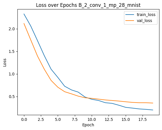
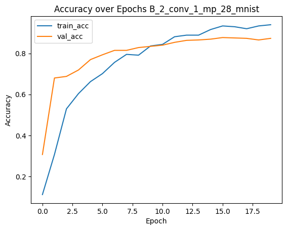
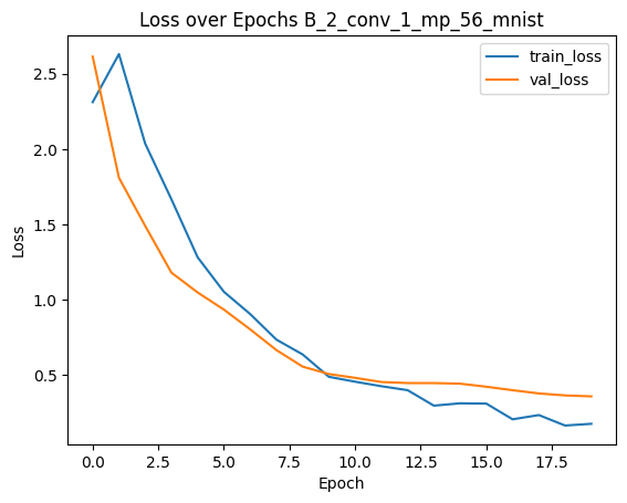
Model Architectures
Our experiments use two distinct neural network architectures trained on the MNIST dataset at each resolution:
Convolutional Neural Network (CNN): Models with prefix ‘B_2_conv_1_mp’ contain 2 convolutional layers followed by a max pooling layer Multi-Layer Perceptron (MLP): Models with prefix ‘A_1_128’ consist of a single hidden layer with 128 neurons
This gives us 4 model configurations in total:
- CNN at 28×28 resolution
- MLP at 28×28 resolution
- CNN at 56×56 resolution
- MLP at 56×56 resolution
data   = collect_data(IMAGE_SIZES)
models = collect_models(data)
comparing all models with fgsm method
We will now visualize how model accuracy changes as we increase the perturbation magnitude \(\epsilon\):
def compare_models_with_fgsm(models: list[ModelMeta], data: List[DataMeta]):
    """
    Compare model accuracy under FGSM attacks.

    Args:
        models: List of ModelMeta holding model and metadata.
        data: List of DataMeta containing test datasets.

    Returns:
        results: Dictionary mapping model names to lists of accuracies
                 at each epsilon value.
        examples: Dictionary mapping model names to lists of adversarial
                  example batches (first 5 examples per epsilon).
    """
    print("Compare models with fgsm")

    n_row_examples = 5
    examples = {m.name: [] for m in models}
    results  = {m.name: [] for m in models}

    for m in tqdm(models, desc="FGSM on Models"):
        d = data[m.data_ofs]
        assert d.test_ds is not None

        for eps in tqdm(EPSILONS, desc=f"Eps: {m.name}"):
            cfg = AttackConfig(victim=m.model, epsilon=eps,
                               attack_fn=fgsm_attack,
                               norm_fn=normalize,
                               dnorm_fn=denormalize)
            advs = adversarial_attack(cfg, d.test_ds)
            acc = evaluate_adversarial(advs)[0]
            results[m.name].append(acc)
            examples[m.name].append(advs[:n_row_examples])

    return results, examples
results, examples = compare_models_with_fgsm(models, data)
plot_diff_model_robustness_eps(models, results, "A", "fgsm")
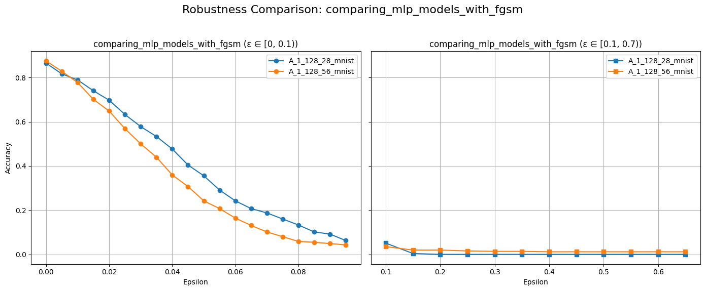
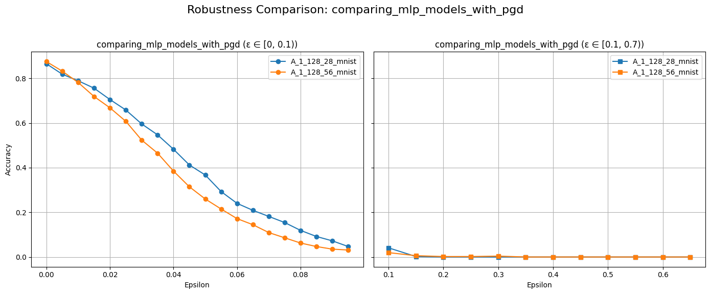
The plot above should show a decline in model accuracy as \(\epsilon\) increases. This is expected because larger perturbations make it easier to push examples across decision boundaries. We typically observe that accuracy starts near the clean test accuracy when \(\epsilon\) is close to zero and gradually decreases as \(\epsilon\) grows.
Our results also indicate that the MLP model (A_1_128_56) exhibits a steeper decline in accuracy compared to our smaller model as \(\epsilon\) increases.
print(models[0].name)
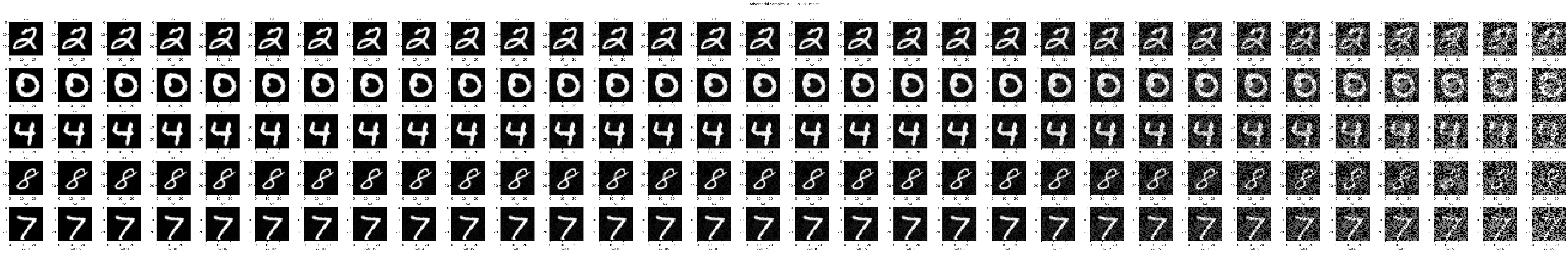
title = f"Adversery Examples with FGSM: Model {models[0].name}"
plot_adv_example_eps_or_c(examples, EPSILONS, models[0].name, title)
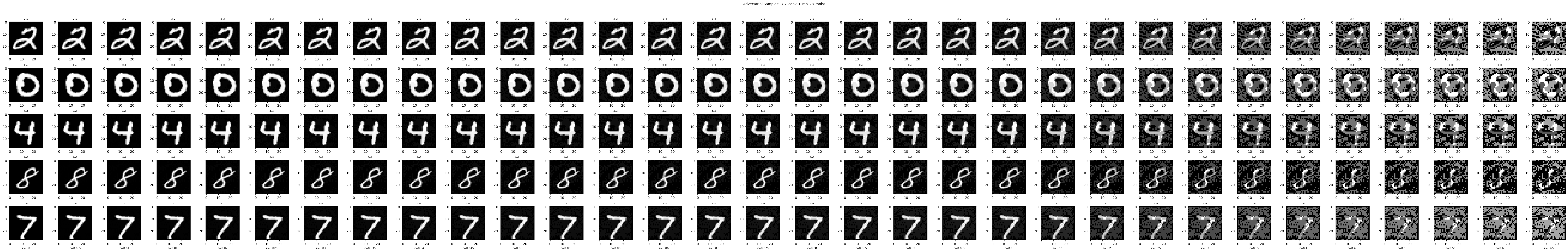
Let’s also examine the visual appearance of adversarial examples for our first model:
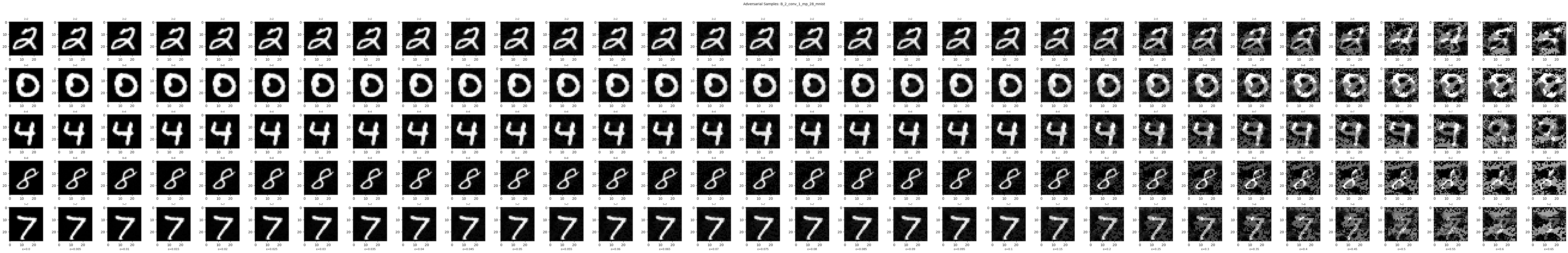
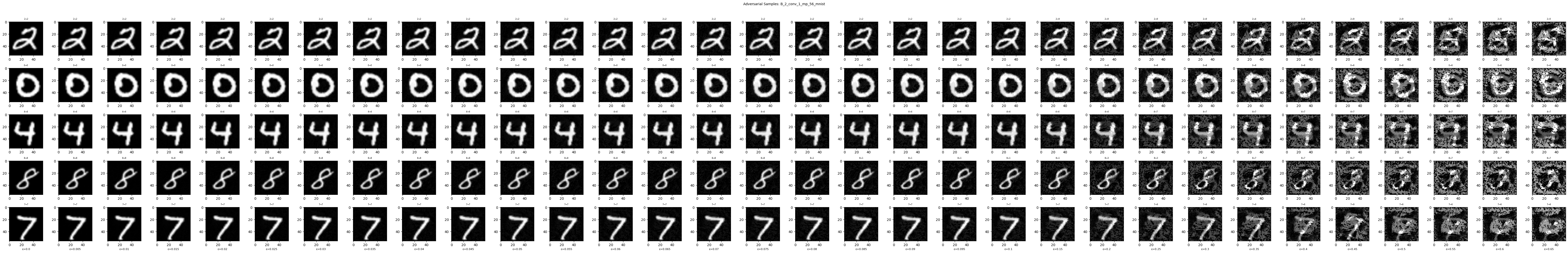
In these visualizations, we observe that as \(\epsilon\) increases, the perturbations become more visible to the human eye. For small values of \(\epsilon\) (e.g., 0.01-0.05), the adversarial examples look nearly identical to the original images. At larger values (e.g., 0.2-0.3), we start to see visible noise patterns that distort the original image while still preserving its general appearance.
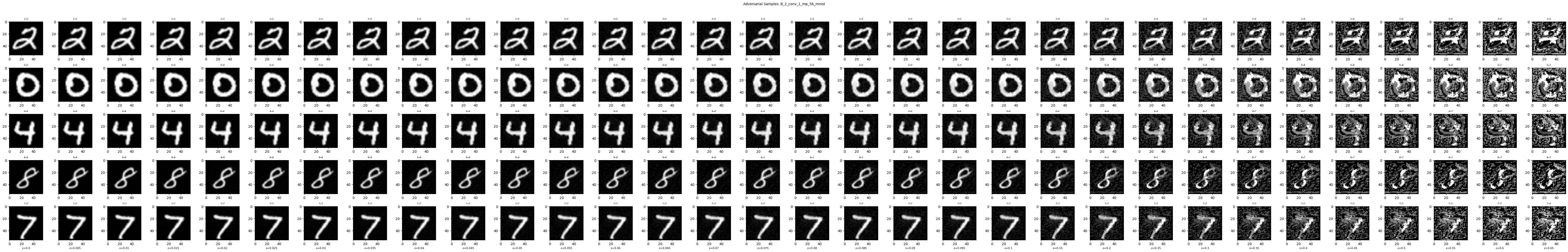
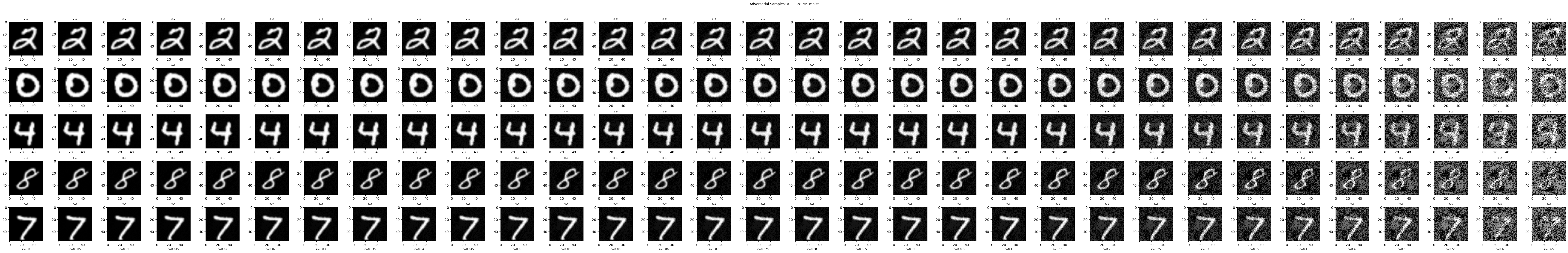
title = f"Adversery Examples with FGSM: Model {models[1].name}"
plot_adv_example_eps_or_c(examples, EPSILONS, models[1].name, title)
plot_diff_model_robustness_eps(models, results, "B", "fgsm")
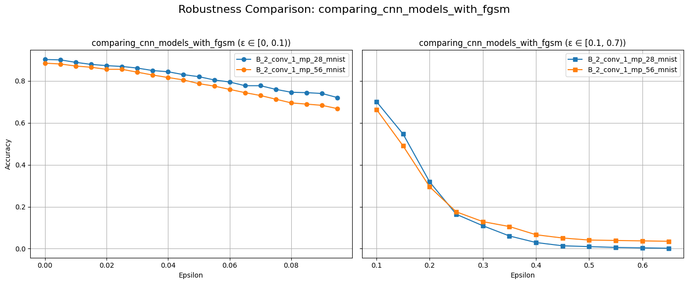
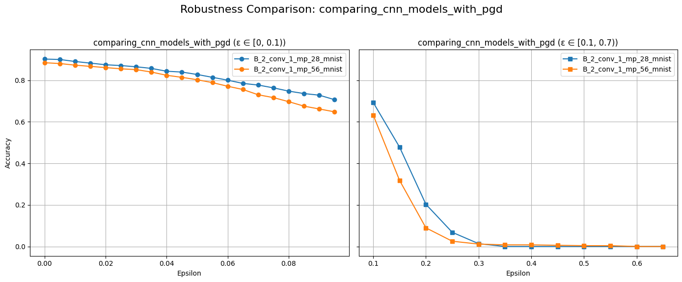
For Group B models, we observe different robustness characteristics compared to Group A. It seems that the CNN models are inherently more robust.
title = f"Adversery Examples with FGSM: Model {models[2].name}"
plot_adv_example_eps_or_c(examples, EPSILONS, models[2].name, title)
title = f"Adversery Examples with FGSM: Model {models[3].name}"
plot_adv_example_eps_or_c(examples, EPSILONS, models[3].name, title)
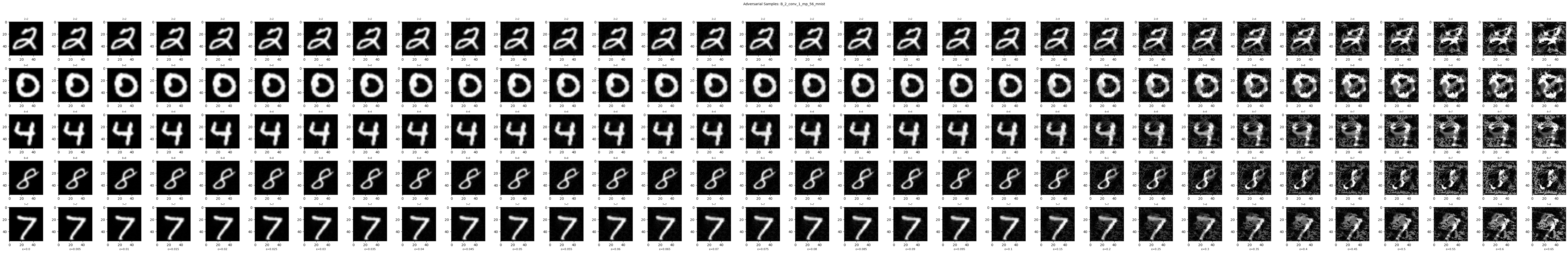
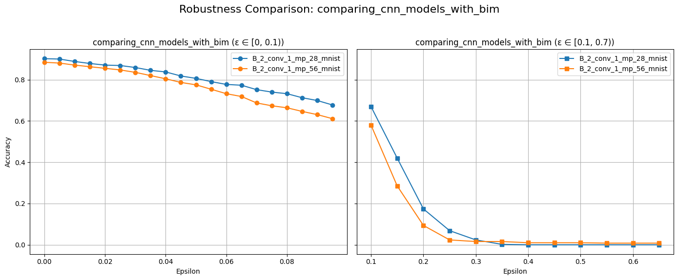
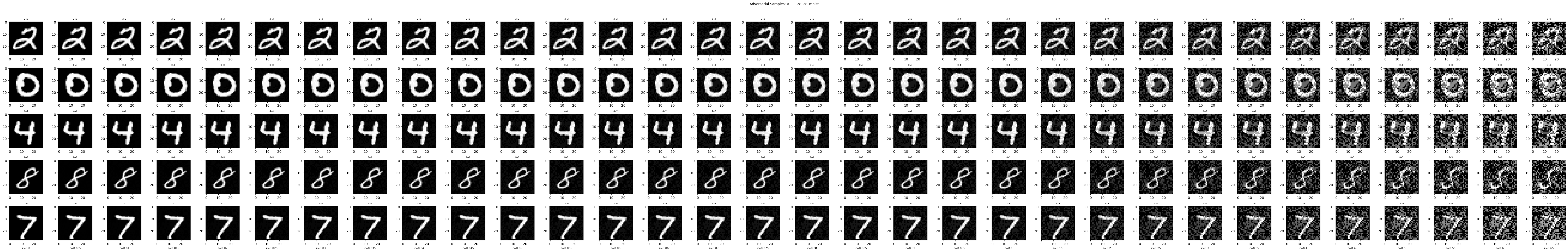
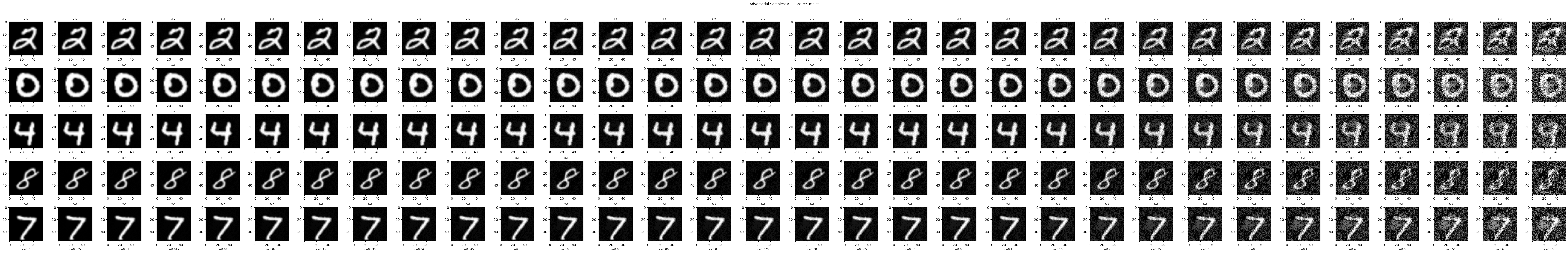
comparing all models with bim method
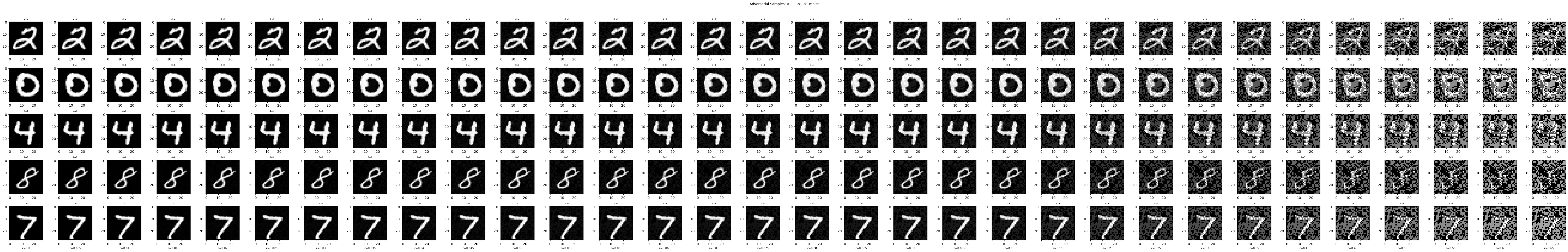
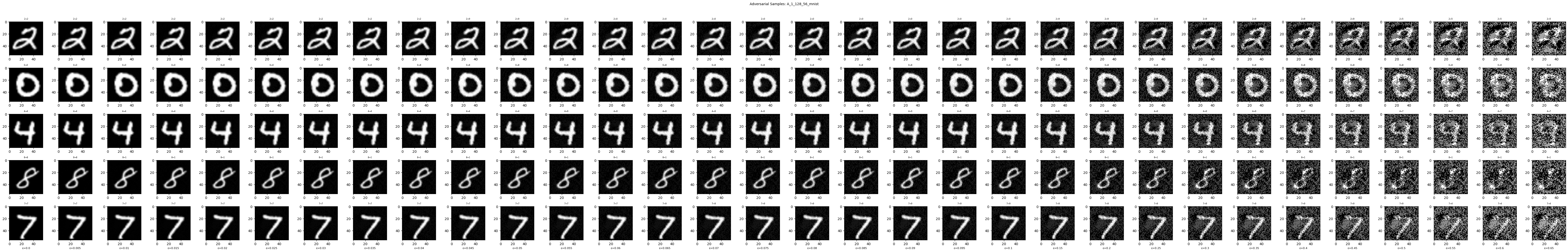
Now we’ll visualize the effectiveness of BIM attacks:
def compare_models_with_bim(models: List[ModelMeta], data: List[DataMeta]):
    """
    Compare model accuracy under Basic Iterative Method (BIM) attacks.

    BIM applies FGSM iteratively for a fixed number of steps.

    Args:
        models: List of ModelMeta.
        data: List of DataMeta.

    Returns:
        results: Accuracies per epsilon.
        examples: Sample adversarial batches.
    """
    print("Compare models with bim")

    steps = 10

    results  = {m.name: [] for m in models}
    examples = {m.name: [] for m in models}

    for m in tqdm(models, desc="BIM on Models"):
        d = data[m.data_ofs]
        assert d.test_ds is not None

        for eps in tqdm(EPSILONS, desc=f"Eps: {m.name}"):
            alpha = eps / steps

            cfg = AttackConfig(victim=m.model, epsilon=eps,
                               alpha=alpha, steps=steps,
                               attack_fn=bim_attack,
                               norm_fn=normalize,
                               dnorm_fn=denormalize)
            advs = adversarial_attack(cfg, d.test_ds)
            acc = evaluate_adversarial(advs)[0]
            results[m.name].append(acc)
            examples[m.name].append(advs[:5])

    return results, examples
results, examples = compare_models_with_bim(models, data)
plot_diff_model_robustness_eps(models, results, "A", "bim")
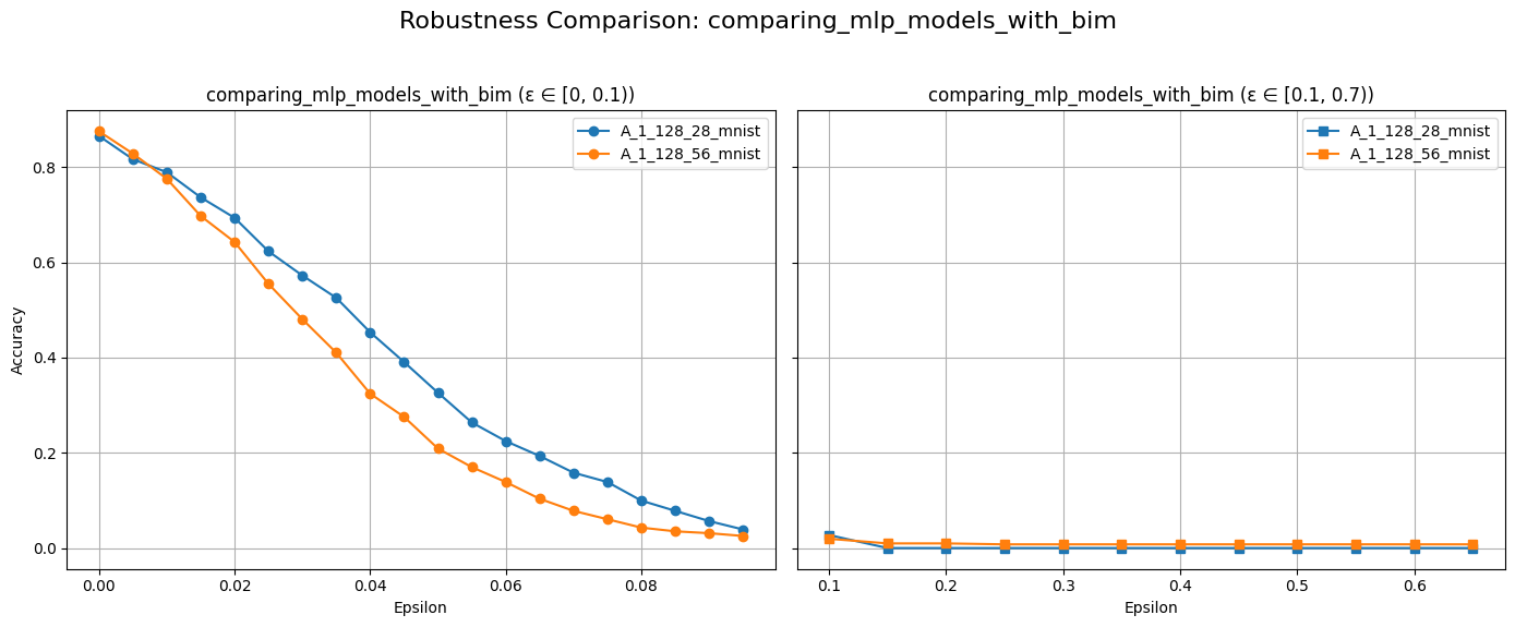
Compared to FGSM, we observe that BIM generally achieves lower model accuracy at the same \(\epsilon\) values. This is because the iterative nature of BIM allows it to find more optimal adversarial examples.
title = f"Adversery Examples with BIM: Model {models[0].name}"
plot_adv_example_eps_or_c(examples, EPSILONS, models[0].name, title)
title = f"Adversery Examples with BIM: Model {models[1].name}"
plot_adv_example_eps_or_c(examples, EPSILONS, models[1].name, title)
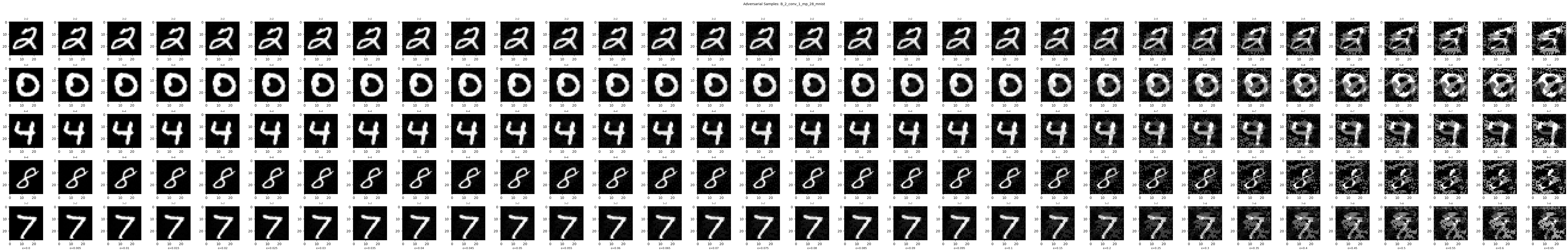
plot_diff_model_robustness_eps(models, results, "B", "bim")
title = f"Adversery Examples with BIM: Model {models[2].name}"
plot_adv_example_eps_or_c(examples, EPSILONS, models[2].name, title)
title = f"Adversery Examples with BIM: Model {models[3].name}"
plot_adv_example_eps_or_c(examples, EPSILONS, models[3].name, title)
comparing all models with pgd method
Now we’ll visualize the effectiveness of PGD attacks:
def compare_models_with_pgd(models: List[ModelMeta], data: List[DataMeta]):
    """
    Compare model accuracy under Projected Gradient Descent (PGD) attacks.

    PGD = BIM + projection step to enforce L-infinity constraint.

    Returns:
        results: Accuracy drop per epsilon.
        examples: Adversarial example batches.
    """
    print("Compare models with pgd")

    steps = 10

    results  = {m.name: [] for m in models}
    examples = {m.name: [] for m in models}

    for m in tqdm(models, desc="PGD on Models"):
        d = data[m.data_ofs]
        assert d.test_ds is not None

        for eps in tqdm(EPSILONS, desc=f"Eps: {m.name}"):
            alpha = eps / steps

            cfg = AttackConfig(victim=m.model, epsilon=eps,
                               alpha=alpha, steps=steps,
                               attack_fn=pgd_attack,
                               norm_fn=normalize,
                               dnorm_fn=denormalize)
            advs = adversarial_attack(cfg, d.test_ds)
            acc = evaluate_adversarial(advs)[0]
            results[m.name].append(acc)
            examples[m.name].append(advs[:5])
    return results, examples
results, examples = compare_models_with_pgd(models, data)
plot_diff_model_robustness_eps(models, results, "A", "pgd")
title = f"Adversery Examples with PGD: Model {models[0].name}"
plot_adv_example_eps_or_c(examples, EPSILONS, models[0].name, title)
title = f"Adversery Examples with PGD: Model {models[1].name}"
plot_adv_example_eps_or_c(examples, EPSILONS, models[1].name, title)
plot_diff_model_robustness_eps(models, results, "B", "pgd")
title = f"Adversery Examples with PGD: Model {models[2].name}"
plot_adv_example_eps_or_c(examples, EPSILONS, models[2].name, title)
title = f"Adversery Examples with PGD: Model {models[3].name}"
plot_adv_example_eps_or_c(examples, EPSILONS, models[3].name, title)
comparing all models with cw method
Now we’ll visualize the effectiveness of CW attacks:
def compare_models_with_cw(models: List[ModelMeta], data: List[DataMeta]):
    """
    Compare models under Carlini & Wagner L2 attacks.

    Args:
        models: List of ModelMeta.
        data: List of DataMeta.

    Returns:
        results_acs: Attack success rate (1 - accuracy).
        results_dst: L2 distortions for each constant c.
        examples: Adversarial batches.
    """
    print("Compare models with cw")

    steps = 3000 # cange this!!!
    # c     = 100
    # c > 1 => adversary more imporant than subtle,
    # c < 1 => subtle pertubration more important than finding adversary

    kappa = 0      # not interested in finding strong adversaries
    lr    = 0.001  # default learning rate of the adam solver (SGD)

    results_acs  = {m.name: [] for m in models}
    results_dst  = {m.name: [] for m in models}
    examples     = {m.name: [] for m in models}

    for m in tqdm(models, desc="CW on Models"):
        d = data[m.data_ofs]
        assert d.test_ds is not None

        # TODO(Ibrahim)
        # run each c as seperate process
        for c in tqdm(C, desc=f"C: {m.name}"):
            cfg = AttackConfig(victim=m.model, steps=steps,
                               c=c, kappa=kappa, lr=lr,
                               attack_fn=cw_attack,
                               norm_fn=normalize,
                               dnorm_fn=denormalize)
            advs = adversarial_attack(cfg, d.test_ds)
            acc = evaluate_adversarial(advs)[0]
            results_acs[m.name].append(1 - acc)
            results_dst[m.name].append(cfg.l2)
            examples[m.name].append(advs[:5])

    return results_acs, results_dst, examples
results_acs, results_dst, examples = compare_models_with_cw(models, data)
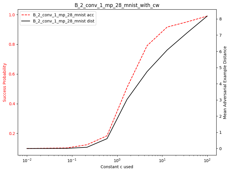
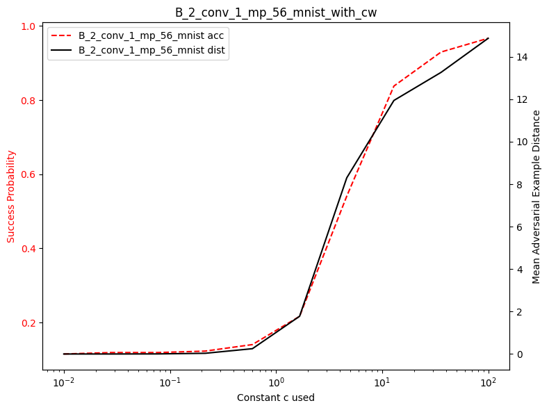
The following plots show both attack success rate (left y-axis) and L2 distortion (right y-axis) as functions of the constant \(c\). We observe that:
As \(c\) increases, the attack success rate increases because more emphasis is placed on finding successful adversarial examples. As \(c\) increases, the L2 distortion also increase because less emphasis is placed on minimizing the perturbation size.
plot_diff_model_robustness_c(results_acs, results_dst, C, "cw")
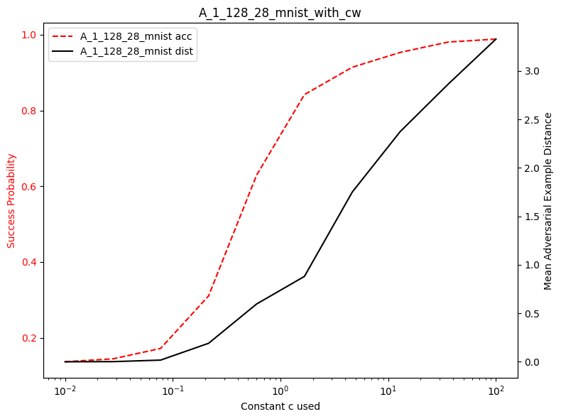
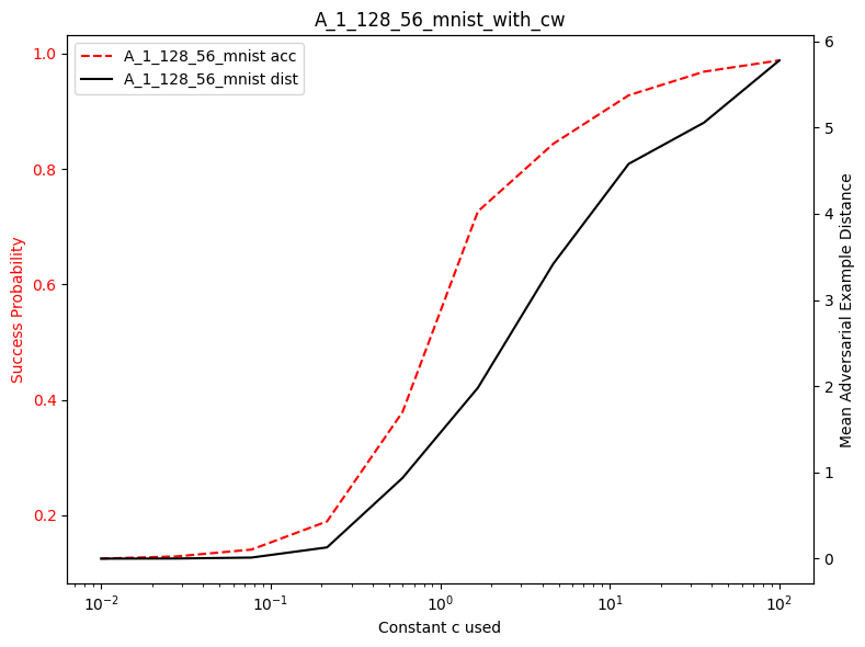
In the following image, we see that the effect of c from the original paper is somewhat similar to our findings.
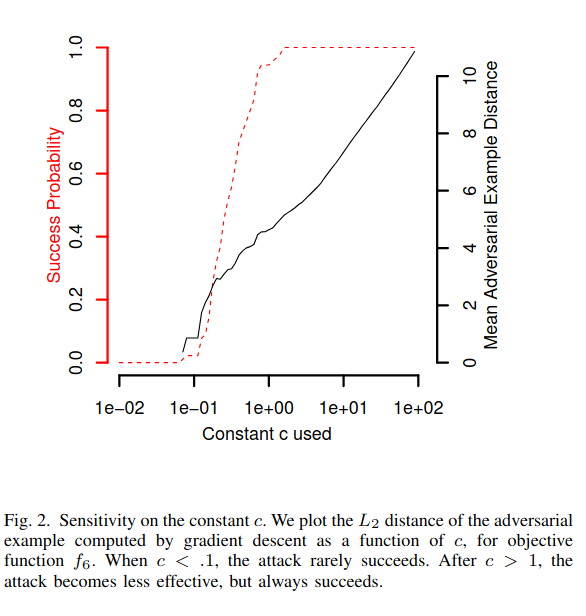
We see that we are somewhat close, as we don’t exactly have the same models as well.
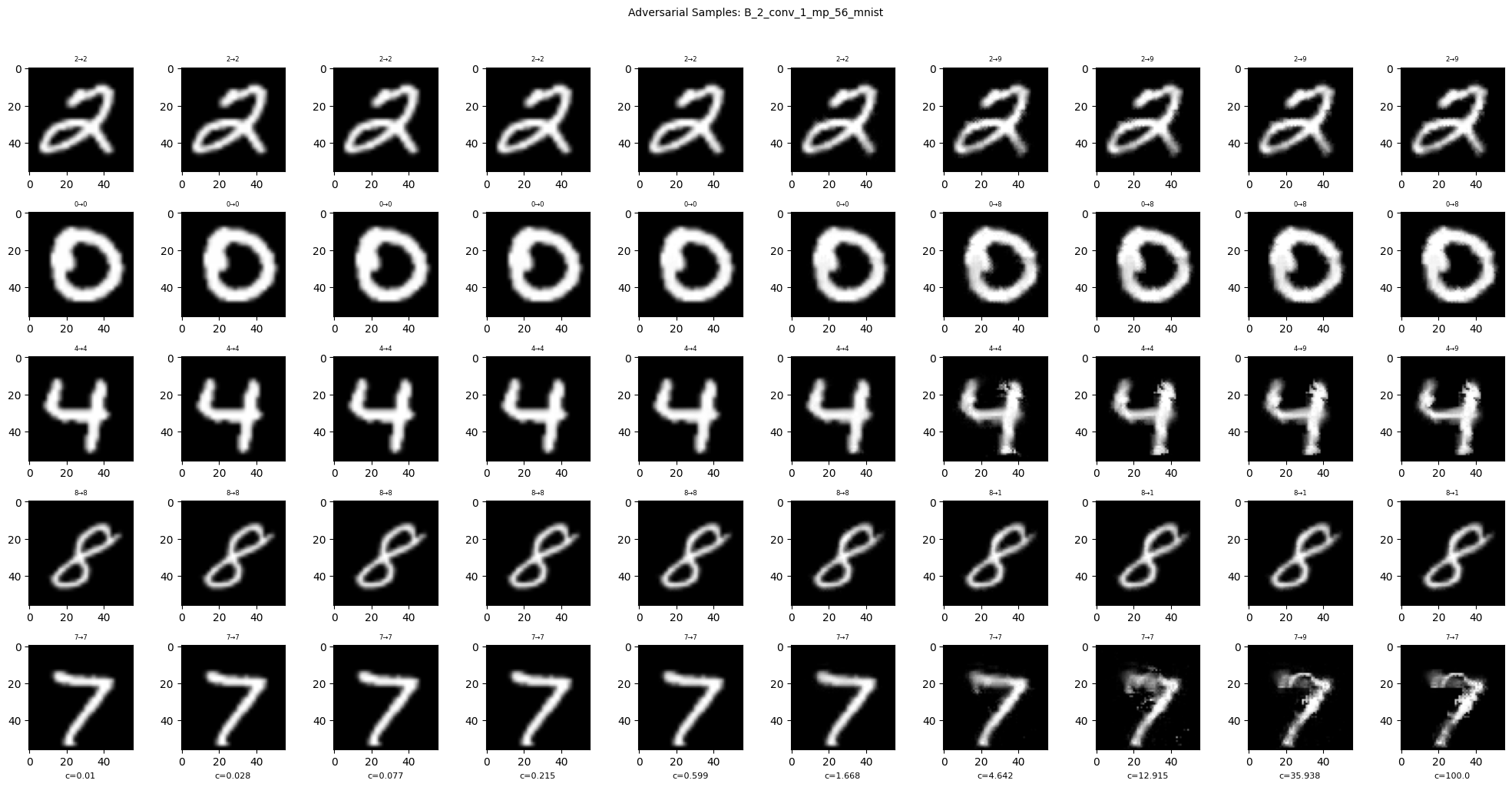
title = f"Adversery Examples with CW: Model {models[0].name}"
plot_adv_example_eps_or_c(examples, C, models[0].name, title, symbol='c')
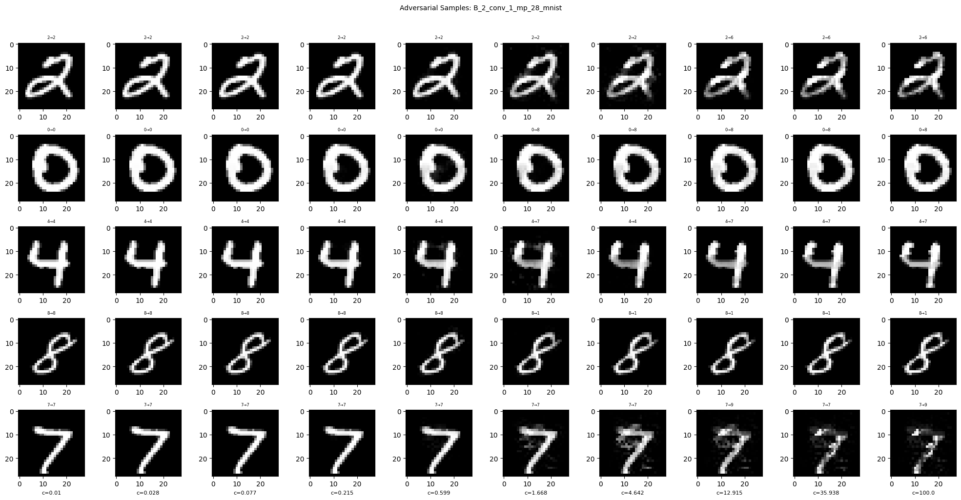
The C&W attack, which is optimization-based has minimal perturbations. Highly effective but computationally intensive…
title = f"Adversery Examples with CW: Model {models[1].name}"
plot_adv_example_eps_or_c(examples, C, models[1].name, title, symbol='c')
5.5 Adversarial Generative Attack Methods
Classic methods as seen in the previous section, solve an optimization for each image. Minimizing a loss and a norm penalty. They work well but are slow, since you have to run the model multiple times per input.
A. Generative Perturbations
We train a generator f that maps any natural image to an adversarial example. We want \(x + f(x)\) close to x under some distance d, yet misclassified
B. Preparing Pascal VOC
Pascal VOC is a multi-label dataset, images often contain several object classes. To combat its imbalance, we use repeat-factor sampling.
def collect_voc_data(size, gray=False, datatype=tf.float32) -> DataMeta:
    """
    Load and preprocess Pascal VOC classification data with repeat factor sampling.

    1. Load image-label dataframe.
    2. Compute repeat factor per image:
        - Class frequency f_c = P(class c)
       - Repeat factor r_c = max(1, sqrt(t / f_c)); t is threshold (e.g., 0.10).
    3. Duplicate images based on maximum repeat factor across their labels.
    4. Build training and validation tf.data pipelines.

    Args:
        size: Target image height and width.
        gray: Convert to grayscale if True.
        datatype: Tensor dtype for images and labels.

    Returns:
        DataMeta with train_ds, val_ds, and no test_ds.
    """
    print("Loading from hard disk")

    train_df, labels = load_training_set()
    train_set, val_set = train_test_split(
        train_df,
        test_size=0.2,
        random_state=42,
        shuffle=True
    )

    print("Calculating repeat factor...")

    label_names = labels.tolist()
    train_labels = train_set[label_names].values.astype(np.float32)
    val_labels   = val_set[label_names].values.astype(np.float32)

    t = 0.10
    class_freq   = train_labels.mean(0)
    r_c          = np.maximum(1.0,np.sqrt(t / np.clip(class_freq, 1e-12, None)))

    repeat_factors = []
    for row in train_labels:
        present = np.where(row == 1)[0]
        repeat_factors.append(
            int(np.ceil(r_c[present].max())) if len(present) else 1
        )

    train_img_paths, train_seg_paths, train_labels = [], [], []
    for (idx, rf) in zip(train_set.index, repeat_factors):
        img_path = f"{base_path}train/img/train_{idx}.npy"
        seg_path = f"{base_path}train/seg/train_{idx}.npy"
        lab_vec  = train_set.loc[idx, label_names].values.astype(np.float32)
        for _ in range(rf):
            train_img_paths.append(img_path)
            train_seg_paths.append(seg_path)
            train_labels.append(lab_vec)

    train_labels    = np.stack(train_labels, axis=0)
    train_img_paths = np.array(train_img_paths)

    train_labels = train_labels[:NUM_TRAIN_IMAGES]
    train_img_paths = train_img_paths[:NUM_TRAIN_IMAGES]

    print(f"total amount of training images: {len(train_img_paths)}")

    print("Loading training repeated images...")
    # FIXME(Ibrahim)
    # training False because we don't want to augment.
    # because it doesn't respect the batch_size
    # at:dag
    train_cls_ds = make_cls_dataset(train_img_paths, train_labels,
                                    batch_size=BATCH_SIZE, training=False)
                                    # normalize=True, size=(size, size),
                                    # x_dtype=datatype, y_dtype=datatype,
                                    # grayscale=gray)

    val_img_paths = [f"{base_path}train/img/train_{idx}.npy" for idx in val_set.index]

    val_labels    = val_labels[:NUM_VAL_IMAGES]
    val_img_paths = val_img_paths[:NUM_VAL_IMAGES]

    print(f"total amount of validation images: {len(val_img_paths)}")

    print("Loading validation repeated images...")

    val_cls_ds   = make_cls_dataset(val_img_paths, val_labels,
                                    batch_size=BATCH_SIZE, training=False)
                                    # normalize=True, size=(size, size),
                                    # x_dtype=datatype, y_dtype=datatype,
                                    # grayscale=gray)

    dm = DataMeta(size=size,
                  labels=labels.to_list(),
                  name="voc",
                  train_ds=train_cls_ds,
                  val_ds=val_cls_ds,
                  test_ds=None)
    return dm
C. The Target: EfficientNetV2-L
Our best classification model was based on the EfficientNetV2-L.
def get_best_model(size, num_classes):
    """
    Load the best-performing MultiLabelClassificationModel with EfficientNetV2-L backbone.

    This function builds the model architecture,
    loads pretrained weights from disk, and returns a compiled model instance.

    Args:
        size : Height and width of the input images (assumed square).
        num_classes : Number of output classes for the classification task.

    Returns:
        model : A Keras model instance with loaded weights, ready for inference or further training.
    """
    class_eff_large_model = MultiLabelClassificationModel(
        backbone_name="EfficientNetV2L",
        input_shape=(size, size, 3),
        hidden_units=512,
        dropout_rate=0.2,
        freeze_backbone=True,
        num_classes=num_classes
    )

    path = f'{xo_path}/class_eff_model.weights.h5'
    class_eff_large_model.load_weights(path)
    return class_eff_large_model
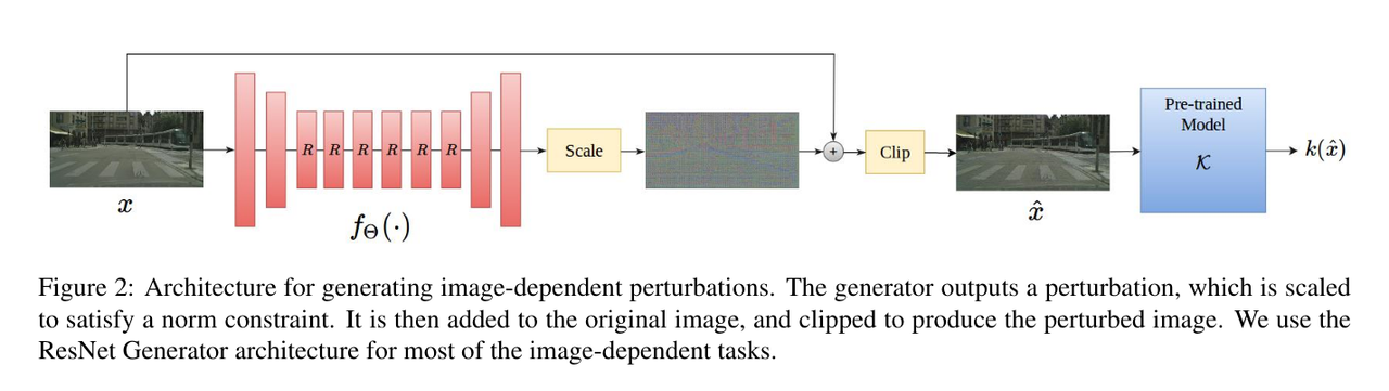
D. Building the Adversarial Generator
We design a ResNet-style encoder–decoder that, given \(x\), outputs a \(delta\)
in [−1,1] via a tanh:
class ReflectionPadding2D(tf.keras.Layer):
    """
    Custom layer for reflection padding.

    Pads the input tensor along height and width dimensions by reflecting the border values.

    Args:
        padding : Number of rows and columns to pad on each side.
    """
    def __init__(self, padding=(1, 1), **kwargs):
        """TODO."""
        self.padding = tuple(padding)
        self.input_spec = [tf.keras.InputSpec(ndim=4)]
        super(ReflectionPadding2D, self).__init__(**kwargs)

    def compute_output_shape(self, s):
        """If you are using "channels_last" configuration."""
        return (s[0], s[1] + 2 * self.padding[0], s[2] + 2 * self.padding[1], s[3])

    def call(self, x, mask=None):
        """TODO."""
        w_pad,h_pad = self.padding
        return tf.pad(x, [[0,0], [h_pad,h_pad], [w_pad,w_pad], [0,0] ], 'REFLECT')

def attacker_model(image_size, input_nc=1, ngf=64, n_blocks=6):
    """
    Builds a ResNet-based perturbation generator.

    The generator takes an input image and outputs a small "delta" image (perturbation)
    that, when added to the input, creates an adversarial example.

    Architecture overview:
    ----------------------
    1. Initial 7x7 convolution with reflection padding
    2. Two downsampling conv layers (stride=2)
    3. n_blocks residual blocks
    4. Two upsampling transposed conv layers
    5. Final 3x3 conv to produce a single-channel delta

    Args:
        image_size : Height and width of the (square) input images.
        input_nc : Number of input channels (e.g., 1 for grayscale, 3 for RGB).
        ngf : Base number of generator filters.
        n_blocks : Number of ResNet blocks in the middle of the network.

    Returns:
        model : Keras Model mapping input image to delta perturbation.
    """

    # norm and bias settings
    norm_layer = tf.keras.layers.BatchNormalization
    act_layer = tf.keras.layers.ReLU

    # input
    img_in = tf.keras.layers.Input(shape=(image_size, image_size, input_nc))

    # initial convolution
    x = ReflectionPadding2D((3, 3))(img_in)
    # x = tf.keras.layers.ZeroPadding2D((3, 3))(img_in)
    x = tf.keras.layers.Conv2D(ngf, 7, padding='valid')(x)
    x = norm_layer()(x)
    x = act_layer()(x)

    # downsampling
    x = tf.keras.layers.Conv2D(ngf * 2, 3, strides=2, padding='same')(x)
    x = norm_layer()(x)
    x = act_layer()(x)
    x = tf.keras.layers.Conv2D(ngf * 4, 3, strides=2, padding='same')(x)
    x = norm_layer()(x)
    x = act_layer()(x)

    # ResNet blocks
    for _ in range(n_blocks):
        pad = 1
        y = ReflectionPadding2D((pad, pad))(x)
        # y = tf.keras.layers.ZeroPadding2D((pad, pad))(x)
        y = tf.keras.layers.Conv2D(ngf * 4, 3, padding='valid')(y)
        y = norm_layer()(y)
        y = act_layer()(y)
        y = ReflectionPadding2D((pad, pad))(y)
        # y = tf.keras.layers.ZeroPadding2D((pad, pad))(y)
        y = tf.keras.layers.Conv2D(ngf * 4, 3, padding='valid')(y)
        y = norm_layer()(y)
        x = tf.keras.layers.add([x, y])

    # upsampling
    x = tf.keras.layers.Conv2DTranspose(ngf * 2, 3, strides=2, padding='same')(x)
    x = norm_layer()(x)
    x = act_layer()(x)
    x = tf.keras.layers.Conv2DTranspose(ngf, 3, strides=2, padding='same')(x)
    x = norm_layer()(x)
    x = act_layer()(x)

    delta = tf.keras.layers.Conv2D(1, 3, activation='tanh', padding='same')(x)
    model = tf.keras.Model(inputs=img_in, outputs=delta, name='resnet_generator')
    return model
E. Adversarial Training Loop
We wrap generator + victim in a custom Keras model:
-
We optimize only the generator.
-
Loss = classification loss (we use a CW-style loss) + L2 regularizer on delta.
class AdversarialAttacker(tf.keras.Model):
    """
    Keras Model combining generator and victim classifier for adversarial training.

    This model:
    1. Generates a perturbation delta
    2. Applies it to the input image
    3. Evaluates the perturbed image on the victim classifier
    4. Computes a total loss: classification loss + L2 norm regularization

    Args:
        attacker : Generator network producing perturbations.
        victim : Pretrained classifier to be attacked.
        loss_fn : Loss function comparing classifier logits to true labels.
        norm_fn : Function to normalize inputs before feeding the victim.
        dnorm_fn : Function to normalize original inputs (mapping to [-1, 2]).
        kappa : Confidence margin for attacks (e.g., in Carlini-Wagner loss).
        lambda_reg : Regularization weight on L2 norm of perturbation.
        one_hot : If True, convert integer labels to one-hot vectors.
        num_classes : Number of classes for one-hot conversion.
        dtype : Numeric type for computations (e.g., tf.float32).
    """
    def __init__(self, attacker, victim, loss_fn, norm_fn, dnorm_fn,
                 kappa=0, lambda_reg=0.1, one_hot=False, num_classes=10,
                 dtype=tf.float32):
        super().__init__()
        self.attacker = attacker
        self.victim = victim
        self.loss_fn = loss_fn
        self.norm_fn = norm_fn
        self.dnorm_fn = dnorm_fn
        self.kappa = kappa
        self.lambda_reg = lambda_reg
        self.one_hot = one_hot
        self.num_classes = num_classes
        self.datatype = dtype

    def compile(self, optimizer): # pyright: ignore
        """
        Prepare the model for training.

        Args:
            optimizer : Optimizer used for updating generator weights.
        """
        super().compile()
        self.optimizer = optimizer
        self.total_loss_tracker = tf.keras.metrics.Mean(name="total_loss")
        self.clf_loss_tracker   = tf.keras.metrics.Mean(name="clf_loss")
        self.l2_loss_tracker    = tf.keras.metrics.Mean(name="l2_loss")

    @property
    def metrics(self):
        """TODO."""
        return [self.total_loss_tracker, self.clf_loss_tracker, self.l2_loss_tracker]

    def train_step(self, data):
        """
        Custom training logic for a single batch.
        """
        x, y = data  # pyright: ignore

        # tf.cast(y, tf.float16) # or do it when making dataset...
        # tf.cast(x, tf.float16) # or do it when making dataset...

        assert x.dtype == self.datatype
        assert y.dtype == self.datatype

        if self.one_hot:
            y = tf.one_hot(y, depth=self.num_classes)

        batch_size = tf.shape(x)[0] # pyright: ignore

        with tf.GradientTape() as tape:
            delta = self.attacker(x, training=True)
            delta = tf.cast(delta, self.datatype)

            dn_x = self.dnorm_fn(x)

            # map range [-1, 2] back to [0, 1]
            raw = dn_x + delta
            scaled = (raw + 1.0) / 3.0
            x_adv = tf.clip_by_value(scaled, 0.0, 1.0)

            x_adv = self.norm_fn(x_adv)

            # x_adv = x_adv * 255
            # x_adv = tf.clip_by_value(x_adv, 0, 255)
            # x_adv = tf.cast(x_adv, tf.uint8)

            logits = self.victim(x_adv, training=False)
            logits = tf.cast(logits, self.datatype)

            clf_loss = tf.reduce_sum(self.loss_fn(logits, y, self.kappa, self.datatype))

            delta_flat = tf.reshape(delta, [batch_size, -1])
            l2_image = tf.reduce_sum(tf.square(delta_flat), axis=1)
            l2_loss = tf.reduce_sum(l2_image)

            # lambda_reg with clf_loss due to numerical stabiltiy if
            # with l2_loss
            total_loss =  clf_loss + self.lambda_reg * l2_loss

        grads = tape.gradient(total_loss, self.attacker.trainable_weights)
        self.optimizer.apply_gradients(zip(grads, self.attacker.trainable_weights))  # pyright: ignore

        batch_size = tf.cast(batch_size, self.datatype)
        self.total_loss_tracker.update_state(total_loss / batch_size)
        self.clf_loss_tracker.update_state(clf_loss / batch_size)
        self.l2_loss_tracker.update_state(l2_loss / batch_size)

        return {
            "loss": self.total_loss_tracker.result(),
            "clf_loss": self.clf_loss_tracker.result(),
            "l2_loss": self.l2_loss_tracker.result(),
        }

    def test_step(self, data):
        """
        Validation logic, identical to train_step but without weight updates.
        """
        x, y = data # pyright: ignore
        if self.one_hot:
            y = tf.one_hot(y, depth=self.num_classes)

        batch_size = tf.shape(x)[0]  # pyright: ignore

        delta = self.attacker(x, training=False)
        delta = tf.cast(delta, self.datatype)

        dn_x = self.dnorm_fn(x)
        x_adv = tf.clip_by_value(dn_x + delta, 0.0, 1.0)
        x_adv = self.norm_fn(x_adv)

        logits = self.victim(x_adv, training=False)
        logits = tf.cast(logits, self.datatype)

        clf_loss = tf.reduce_sum(self.loss_fn(logits, y, self.kappa, self.datatype))

        delta_flat = tf.reshape(delta, [batch_size, -1])
        l2_loss = tf.reduce_sum(tf.square(delta_flat))

        total_loss = clf_loss + self.lambda_reg * l2_loss

        batch_size = tf.cast(batch_size, self.datatype)
        self.total_loss_tracker.update_state(total_loss / batch_size)
        self.clf_loss_tracker.update_state(clf_loss / batch_size)
        self.l2_loss_tracker.update_state(l2_loss / batch_size)

        return {
            "loss": self.total_loss_tracker.result(),
            "clf_loss": self.clf_loss_tracker.result(),
            "l2_loss": self.l2_loss_tracker.result(),
        }

print("AdversarialAttacker ready for compile and training.")
EPOCHS_          = 100 # cahgen to 30
NUM_CLASSES      = 20
IMAGE_SIZE       = 32
BATCH_SIZE       = 516 # damn...
NUM_TEST_IMAGES  = -1  # change to -1!
NUM_TRAIN_IMAGES = -1
NUM_VAL_IMAGES   = -1

input_nc = 3
datatype  = tf.float32
mixed_precision.set_global_policy('float32')

# data = collect_data([IMAGE_SIZE])[0]
data = collect_voc_data(IMAGE_SIZE, gray=False, datatype=datatype)
print("bruh")
E. Experimental Setup and Training
We’ll now configure and train our adversarial attack model.
For this adversarial training, we’ve made several important design choices:
-
Image Size: We use a relatively small image size (32×32) due to VRAM limitations, though larger images would likely produce more effective attacks.
-
Loss Function: We employ a multi-label adaptation of the Carlini-Wagner loss function, which has proven effective for adversarial attacks.
-
Regularization: The lambda_reg parameter controls the trade-off between perturbation magnitude and attack effectiveness.
-
Training Duration: 100 epochs is sufficient for the generator to learn effective perturbation patterns.
-
Optimizer: Adam with a learning rate of 1e-4 provides stable convergence.
The training process optimizes the generator to create perturbations that fool the victim classifier while remaining as small as possible in L2 norm.
attacker_net = attacker_model(IMAGE_SIZE, input_nc=input_nc)
print(attacker_net.input)
print(attacker_net.count_params())
victim_net   = get_best_model(IMAGE_SIZE, NUM_CLASSES)
print(victim_net.model.input)
print(victim_net.model.count_params())
attacker_wrapper = AdversarialAttacker(
    attacker=attacker_net,
    victim=victim_net.model,
    loss_fn=multi_label_loss_cw_fn,
    norm_fn=lambda x:x,
    dnorm_fn=lambda x:x,
    kappa=0,
    lambda_reg=1,
    dtype=datatype
)

attacker_wrapper.compile(optimizer=tf.keras.optimizers.Adam(1e-4))

history = attacker_wrapper.fit(
    data.train_ds,
    validation_data=data.val_ds,
    epochs=EPOCHS_
)

attacker_net.save_weights("attacker_wrapper_100.weights.h5")
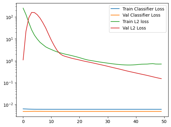
plt.plot(history.history['clf_loss'], label='Train Classifier Loss')
plt.plot(history.history['val_clf_loss'], label='Val Classifier Loss')
plt.legend()
plt.plot(history.history['l2_loss'], label='Train L2 loss ')
plt.plot(history.history['val_l2_loss'], label='Val L2 Loss')
plt.legend()
plt.yscale('log')
save_path = f"{PLOTS_DIR}/loss_plot_best_testing.png"
plt.savefig(save_path)
plt.show()
plt.close()
5.6. Results Analysis
In the loss plot, we see that both losses stabilize, though the classification loss is suspiciously low and the l2 loss is suspiciously high.
counter = 0
examples_for_plot = []
for x_batch, y_batch in data.val_ds:
delta = attacker_wrapper.attacker(x_batch, training=False)
delta = tf.cast(delta, x_batch.dtype)
x_adv = tf.clip_by_value(x_batch + delta, 0.0, 1.0)
orig_logits = victim_net.model(x_batch, training=False)
adv_logits = victim_net.model(x_adv, training=False)
# top 1 accuracy!
orig_preds = tf.argmax(orig_logits, axis=1).numpy()
adv_preds = tf.argmax(adv_logits, axis=1).numpy()
indices = [list(np.where(row == 1)[0]) for row in y_batch]
collection = zip(indices, adv_preds, orig_preds, x_adv.numpy())
for orig, adv, label, img in collection:
examples_for_plot.append((orig, int(adv), label, img))
def evaluate_adversarial(adv_examples):
"""TODO."""
correct = sum(1 for y_true, y_pred, _, _ in adv_examples if y_pred in y_true)
total = len(adv_examples)
return (correct / total) if total > 0 else 0.0
acc = evaluate_adversarial(examples_for_plot)
print("The effectiveness of the attacker model:\n")
print("compare ground truth label with predicted label of adverserial image")
print("high number is bad.")
print(acc)
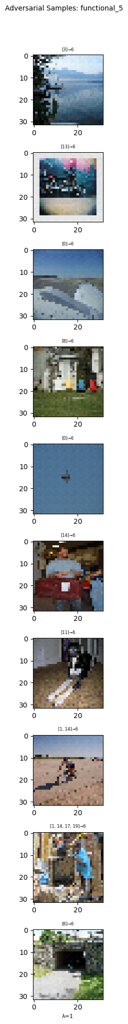
best_lambda = 1
model_name = victim_net.model.name
examples = { model_name: [ examples_for_plot[:10] ] }
eps_or_c = [best_lambda]
plot_adv_example_eps_or_c(
examples=examples,
eps_or_c=eps_or_c,
name=model_name,
title=f"_A_adv_examples_best_lambda_{best_lambda:.0e}",
symbol='λ'
)
import matplotlib.pyplot as plt

x_batch, y_batch = next(iter(data.val_ds))
delta = attacker_wrapper.attacker(x_batch, training=False)
x_adv = tf.clip_by_value(x_batch + delta, 0.0, 1.0)
adv_logits = victim_net.model(x_adv, training=False)
adv_preds   = tf.argmax(adv_logits,  axis=1).numpy()

n_images = 10

x = x_batch.numpy()
d = delta.numpy()
xa = x_adv.numpy()

# scale perturbation for display
d_min, d_max = d.min(), d.max()
d_vis = (d - d_min) / (d_max - d_min + 1e-12)

fig, axes = plt.subplots(n_images, 4, figsize=(12, 9))  # 4 columns now
for i in range(n_images):
    # show images in cols 0-2
    axes[i, 0].imshow(x[i], cmap='gray')
    axes[i, 1].imshow(d_vis[i], cmap='gray')
    axes[i, 2].imshow(xa[i], cmap='gray')

    # hide axes for images
    for j in range(3):
        axes[i, j].axis('off')

    # prepare the label text
    orig_label = y_batch[i].numpy()
    adv_label  = adv_preds[i]
    selected_labels = [label for label, flag in zip(data.labels, orig_label) if flag == 1.0]
    label_text = f"{selected_labels} → {data.labels[adv_label]}"

    # dump the text into the 4th column
    axes[i, 3].axis('off')
    axes[i, 3].text(
        0.5, 0.5,               # center of the cell
        label_text,
        transform=axes[i,3].transAxes,
        ha='center', va='center',
        color='white',
        backgroundcolor='black',
        fontsize=8
    )

# titles on the top row for the first three columns
axes[0, 0].set_title('Original')
axes[0, 1].set_title('Perturbation')
axes[0, 2].set_title('Adversarial')
axes[0, 3].set_title('Label Flip')  # header for your new text column

plt.tight_layout()
# save or show as before
save_path = f"{PLOTS_DIR}/image_plus_perturbation_equals_.png"
plt.savefig(save_path)
plt.show()
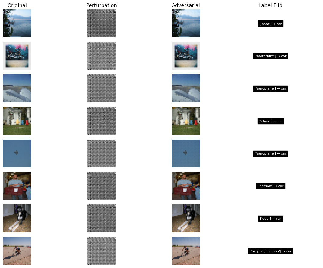
Discussion
This final section of the notebook demonstrated how to build iterative adverserial algorithms and a ResNet generator.
Areas for Improvement:
- Incorporate an adversarial dataset into the classifier’s (and/or segmentation model’s) training process.
- Verify the correct implementation of the victim model to prevent unintended bugs.
Discussion Questions:
-
Is this a realistic attack? Yes, many real-world scenarios grant attackers access to model weights or allow transfer attacks against similar architectures. However, such attacks are only practical in digital pipelines where images are fed directly to the model (e.g., an image hosting service or any other service with a publicly documented face-recognition system).
-
Was the adversary successful? In the generative case presented here, success was limited. Likely due to an implementation issue rather than a fundamental flaw in the methodology. Our iterative approach, however, achieved more reliable attack success.
-
Are the images still recognizable to humans? It depends on the attack parameters: higher-confidence attacks tend to introduce visible artifacts, making the perturbations more noticeable. Lower-confidence attacks can remain imperceptible.
-
Does this mean the original CNN \(h_{\\theta_c}\) is now unreliable? Not necessarily. There are several defensive techniques to bolster model robustness, including:
- Adversarial Training: Augmenting training data with adversarial examples.
- Defensive Distillation: Using knowledge distillation to smooth model gradients.
References:
- Towards Deep Learning Models Resistant to Adversarial Attacks
- Intriguing properties of neural networks
- Generative Adversarial Perturbations
- Towards Evaluating the Robustness of Neural Networks
- The Space of Transferable Adversarial Examples
- EfficientNetV2: Smaller Models and Faster Training
- Universal adversarial perturbations
- Generating Adversarial Examples with Adversarial Networks
- Generative Adversarial Nets
- Towards Deep Learning Models Resistant to Adversarial Attacks