Author: Ibrahim El Kaddouri
Repository:
 The repository is still private, under construction
Introduction
In this report, we will explore the implementation and analysis of various reinforcement learning algorithms within a grid-based game environment. The report begins by explaining some important concepts of RL algorithms, proceeded by some hyperparameter experimentation and concluding with an examination of deep reinforcement learning approaches.
1. Environments and Baselines
1.1 Custom Environment and Random Baseline
This portion focuses on creating a custom environment alongside creating a random agent as a baseline.
goal-seeking environment design
We will implement a goal finding environment where an agent tries to find the goal in a variable size \((n \times m)\) grid-world. The game starts with the player located at \((0, 0)\) and the goal (a cookie) located at \((n − 1, m − 1)\).
The player makes moves until they reach the goal. There are four possible actions: up, down, right and left. Each movement incurs a penalty of \(-1\), while reaching the cookie yields a reward of 0 points.
The state of the agent in this particular environment can be represented by a single number. The environment doesn’t change, thus the agent’s current coordinates provide sufficient state information and satisfies the markov property. In total, there are \(n \times m − 1\) possible states.
Environmental observations are provided to the agent following each action. These observations represent the agent’s current location calculated using the formula:
\[index = current\_row \times ncols + current\_col\]
The environment architecture follows the
OpenAI Gym framework, by
implementing the abstract methods of the class gym.Env, i.e.
reset(), step() and render(). The complete implementation
of the cookie environment can be found in the following file:
src/envs/cookie.py.
random agent baseline
An agent in any kind of environment needs to be able to do two things.
First, perform an action within an environment and second, learn
from previous interactions. Thus, any agent implemented in this report
will have the following two abstract methods implemented: act() and
learn().
We will begin with the random agent as a baseline. A random
agent selects an action uniformly at random, i.e., according to a
uniform distribution. The complete implementation of the random agent
can be found in the following file:
src/baseline/random.py.
performance evaluation
There are different ways to compare the performance of agents. One approach is to compare, for a certain amount of episodes, the evolution of the return of each episode during learning.
The implementation of the training procedure can be found in the following file:
src/tasks/training.py.
evolution of random agent
Using a 5 × 5 instance of the cookie environment, we will plot the
evolution of the average return over an interaction of 10000 episodes by
the random agent.
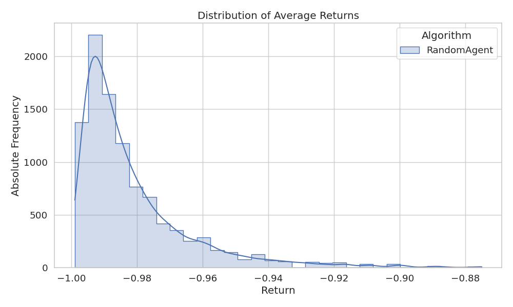
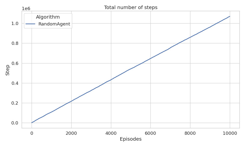
The right figure shows the total number of steps over the 10 000 episodes.
As shown, the average reward is always greater than \(−1\) and less than \(−0.87\) This aligns with expectations: since the agent performs a random walk in the environment, it consistently incurs a step cost of \(−1\) until it reaches the goal, which yields a reward of \(0\).
The accumulated average reward follows this formula:
\[f(\text{steps}) = \frac{\text{steps} -1}{\text{steps}} \quad \text{for} \quad \text{steps} \geq 8\]
Optimally, the agent requires only 8 steps. In that case,
the reward sequence would be: -1, -1, -1, -1, -1, -1, -1, -1, 0.
Averaging this sequence gives \(−8/9 \approx -0.88\),
which is the maximum value observed in the histogram above.
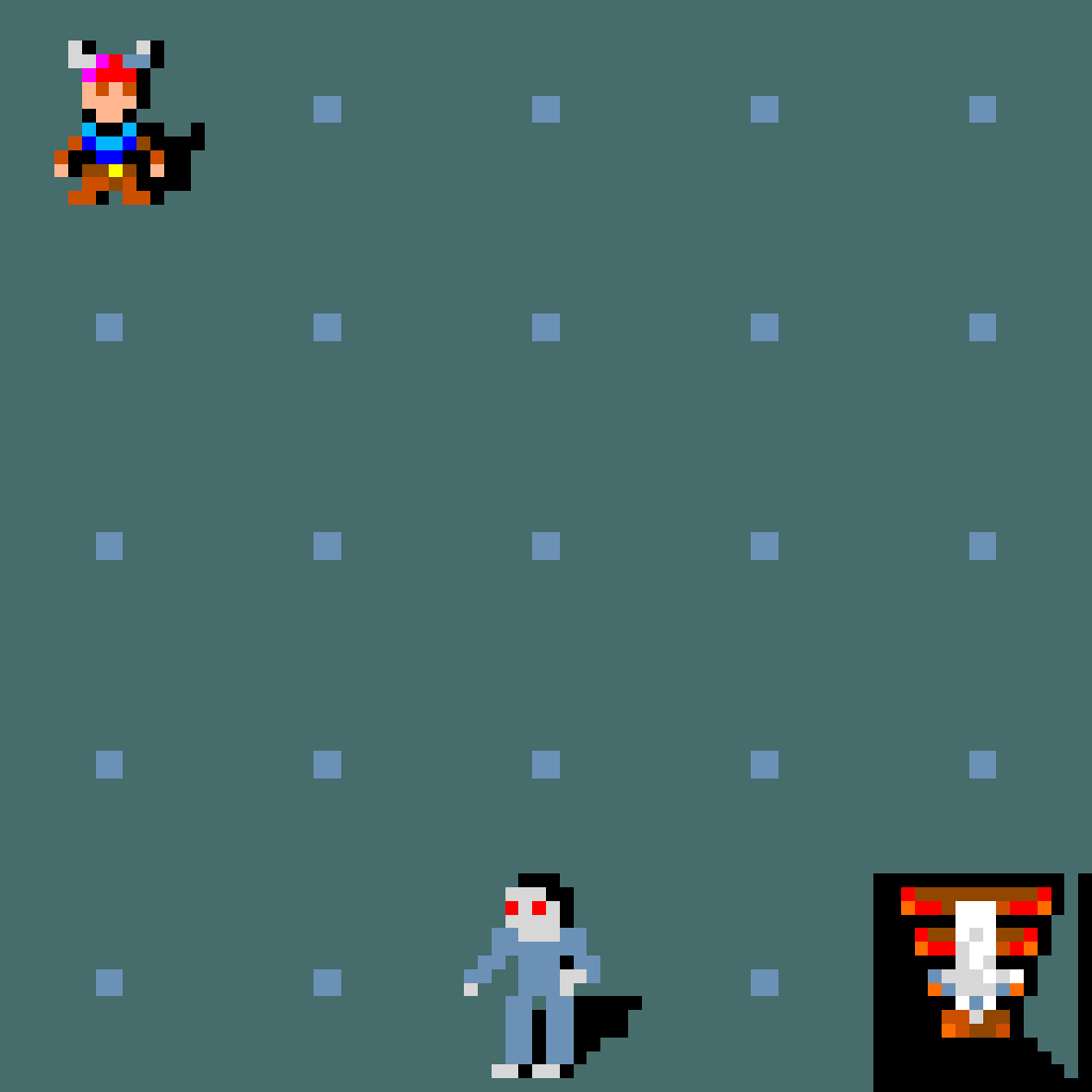
Below, we visualize an episode of the random agent using a GIF:
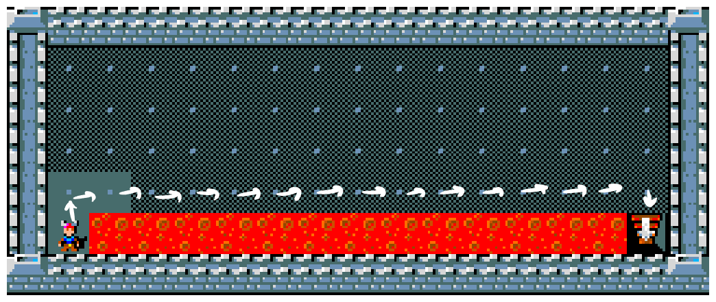
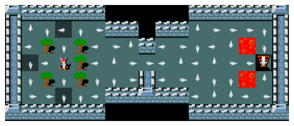
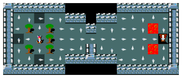
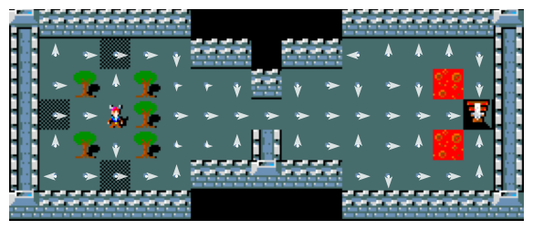
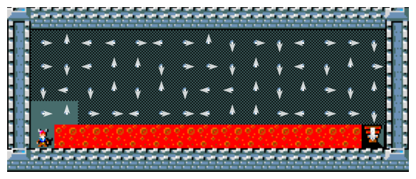
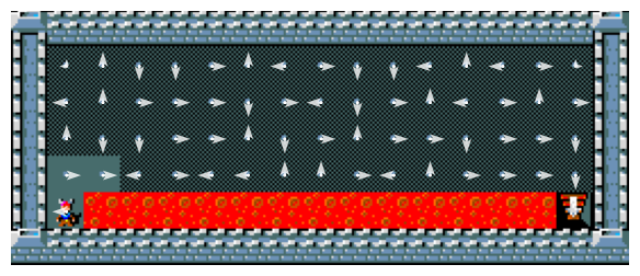
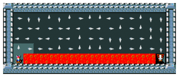
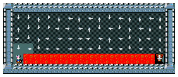
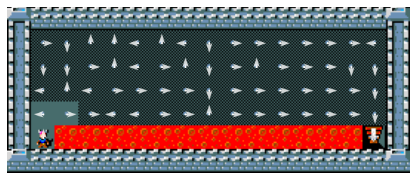
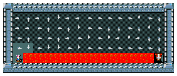
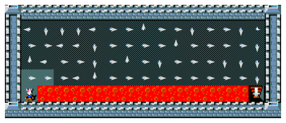
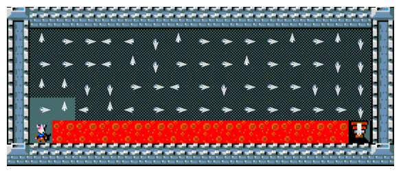
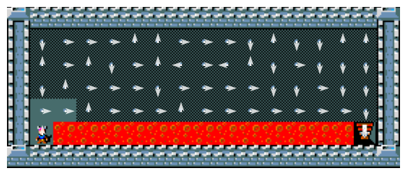
1.2 Minihack environment and fixed baseline
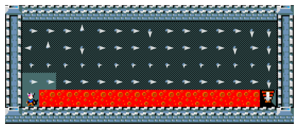
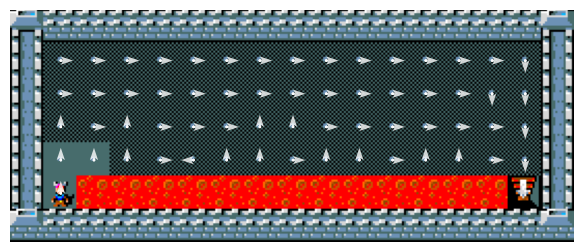
Consider the four Minihack environments in Figure 3. Movement is restricted to cardinal directions (north, south, east, west), matching the previously described cookie environment’s action constraints.
-
EMPTY_ROOMis a simple goal-finding-like environment, where the goal is to reach the downstairs. The agent gets \(−1\) reward for each step. -
CLIFFis based on the cliff-environment by Sutton and Barto. The reward scheme is \(0\) when reaching the goal, \(−1\) for each step. Stepping on the lava gives \(−100\) reward and teleports the agent to the initial state, without resetting the episode. The episode only ends when the goal is reached or the maximum amount of steps is reached -
ROOM_WITH_LAVAis a slightly more complicated goal-finding environment. The reward scheme is the same as theCLIFF. -
ROOM_WITH_MONSTERis an environment identical to theEMPTY_ROOM, but a monster walks around and can attack and kill the agent. The reward scheme is the same as theCLIFFenvironment and \(−100\) for any death.


The implementation of these environments can be found in the following file:
src/envs/rooms.py
fixed agent baseline
We introduce a new baseline for the four environments: the fixed agent. This agent always moves down until it can no longer do so, and then proceeds right. Unlike the random agent, which acts without considering its surroundings, the fixed agent must account for its current position within the environment.
Importantly, we cannot reuse the same state representation as in the cookie environment, since one of the four environments includes a moving object. If only the agent’s position is known, the task becomes partially observed, i.e. it is impossible to fully understand the current environment from only the current agent position.
Take the ROOM_WITH_MONSTER environment as an example.
One possible approach would be to encode the state as a sequence of coordinates,
each representing the position of a moving entity (either the agent or the monster).
However, we opt for a much simpler, though less compact, representation:
the ASCII-based1 NetHack view.
The implementation of the fixed agent is available here:
src/baseline/fixed.py.
evolution of fixed agent
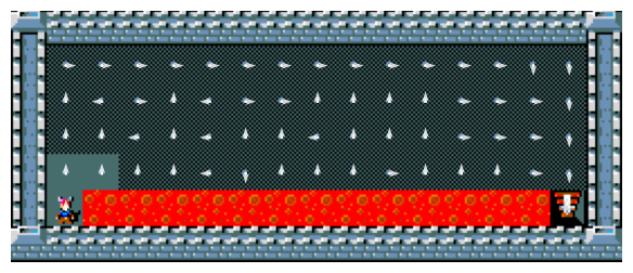
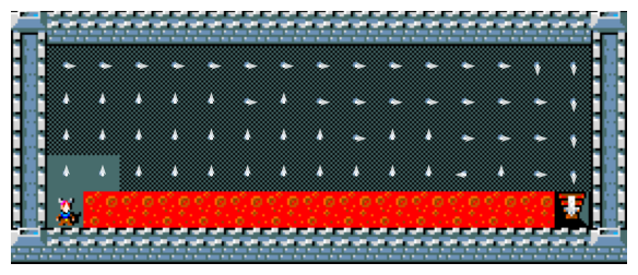
In Figure 4, we visualize the steps
of an episode executed by the fixed agent in the EMPTY_ROOM and
ROOM_WITH_LAVA environments using GIFs.
2. Learning Algorithm Implementation and Analysis
2.1 Algorithmic Experimentation
This portion focuses on implementing various reinforcement learning algorithms and conducting comparative analysis across different environments. Three distinct learning agents have been explored:
-
Monte Carlo On-policy
-
Temporal Difference On-policy (Sarsa)
-
Temporal Difference Off-policy (Q-learning)
All agents utilize \(\epsilon\)-greedy exploration strategies during the learning
phase. The complete implementation of these three agents is located in:
src/algorithms.
on-policy versus off-policy
We will begin by examining the differences between on-policy and off-policy reinforcement learning methods. An algorithm is classified as on-policy when the action used for learning is the same as the action taken during exploration. In contrast, off-policy algorithms maintain separate target and behavior policies.
To compare the two approaches, we use the CLIFF environment to
evaluate the Sarsa and Q-learning algorithms, both employing
\(\epsilon\)-greedy action selection \((\epsilon = 0.1)\).
A constant learning rate \((\alpha = 0.1)\) is used throughout
the experiment. The complete configuration details are available at
src/tasks/config/task2_1.yaml.
The results, shown in Figure 5 and 7, reveal that while Q-learning learns the optimal policy values, its online performance is worse than Sarsa, which instead develops a safer, more indirect route. We’ll break down the reasons below.
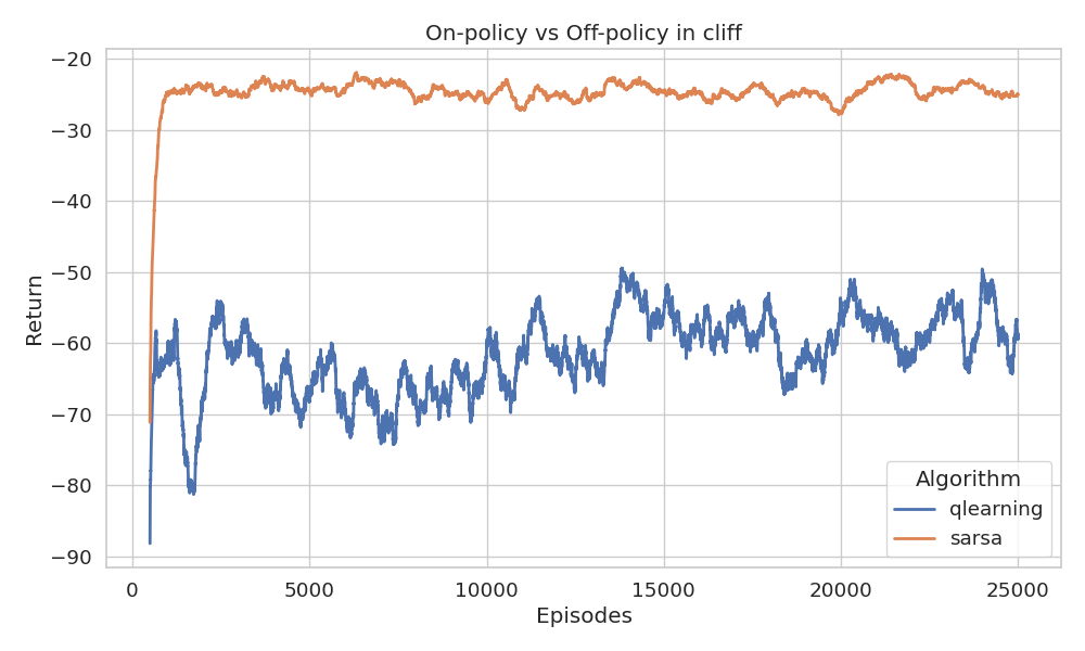
The curve is smoothed using a 500-episode moving average
Theoretically, the maximum cumulative reward obtainable in a single episode corresponds to the following trajectory (starting from the bottom-left corner).
The corresponding reward sequence is -1, -1, ..., -1, 0, resulting in a
return of \(-15\). This is the highest possible return when starting from
the designated starting position. Any deviation from this path, either
through longer trajectories or agent deaths, leads to worse outcomes.
The returns observed during training are shown in Figure 5, smoothed using a moving average. The more negative the return, the more frequently the agent is falling off the cliff, indicating it’s following a riskier path (since cliff falls only happen when navigating close to the lava).
To illustrate the learned strategies, we visualize the policies of both algorithms:
In conclusion, Q-learning develops values for the optimal strategy,
involving choosing actions along the cliff edge. However,
this approach occasionally results in cliff falls due to \(\epsilon\)-greedy
action selection. Sarsa takes action selection into account and learns
a longer but safer pathway through the upper grid region.
monte carlo versus temporal difference analysis
We will highlight the differences between Monte Carlo (MC)
and Temporal Difference (TD) methods using the CLIFF environment.
Specifically, we compare First-Visit MC, Every-Visit MC and TD Sarsa.
All three algorithms are on-policy, so we expect them to learn the same
safe path as observed in the previous experiment.
-
First-Visit MC averages returns following the first visit to a state-action pair within an episode.
-
Every-Visit MC averages returns after every occurrence of that pair in an episode.
For exploration, we use a soft epsilon-greedy policy with
\(\epsilon = 0.4\) and \(\gamma = 1\) for all algorithms
and \(\alpha = 0.1\) for TD. We also average using the
incremental MC
method to improve efficiency which is mathematically equivalent to
sample averaging. The complete configuration details are
available at
src/tasks/config/task2_1.yaml.
We expect both MC methods to converge, but with higher variance compared to TD. TD, however, introduces bias due to bootstrapping, whereas MC methods are (mostly) unbiased. Every-Visit MC does exhibit some bias.
The increased variance in MC arises from estimating the value of a state-action pair based on full returns \(G_t\). The variance of \(G_t\) grows with the episode length 2 and variability of rewards:
\[\operatorname{Var}(G_t) \leq \sum_{k=t+1}^{T} \operatorname{Var}(R_k)\]
In contrast, TD methods update based on the immediate reward \(R_{t+1}\) and the estimated value of the next state:
\[\operatorname{Var}(R_{t+1}) \leq \operatorname{Var}(G_t) \leq \sum_{k=t+1}^{T} \operatorname{Var}(R_k)\]
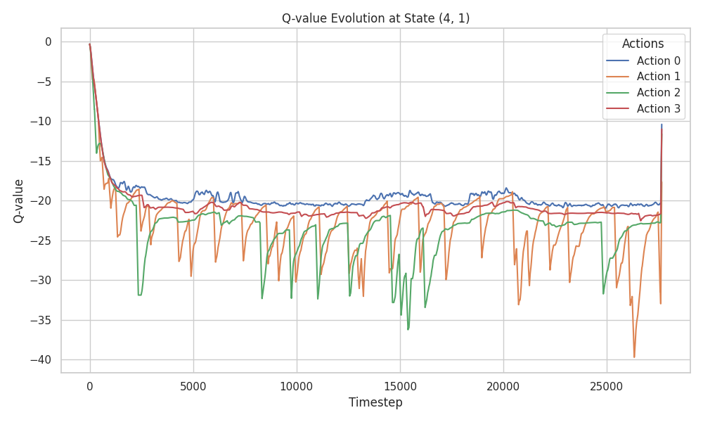
Let’s consider estimating the value of cell \((4,1)\). The agent explores the environment, accumulates rewards or penalties, and uses the sampled returns to update the value estimate of this state.

Using MC methods, the return from (4,1) could be anything,
-100, -200, -1000, or even -15. Each return gets
equal weight in the final estimate. This explains the
high variance in MC methods. TD, on the other hand,
updates using only the immediate reward (between -100 and -1),
resulting in much smaller update variance, especially since
neighbor state values are initialized to 0, and the learning
rate \(\alpha\) reduces the magnitude further.
We validate this observation by examining the Q-value history for state \((4,1)\) across all three algorithms:
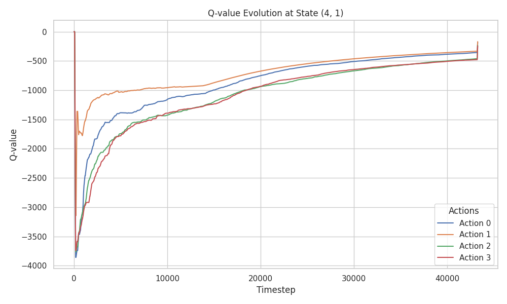
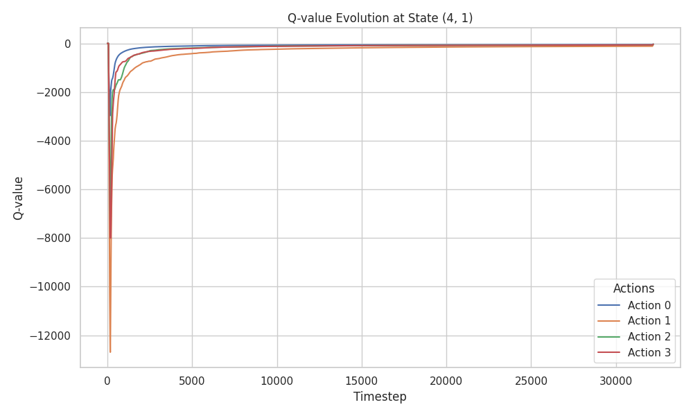
Despite the variance, all three algorithms converge toward the suboptimal, safe policy. This is further confirmed by examining the learned policy maps:

Finally, we present the return and steps per episode evolution:
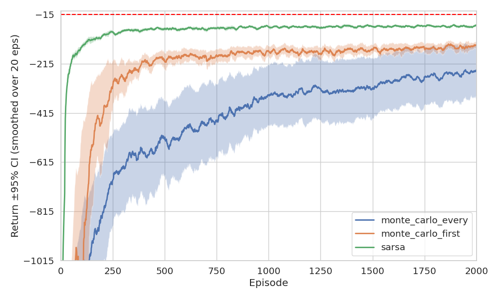
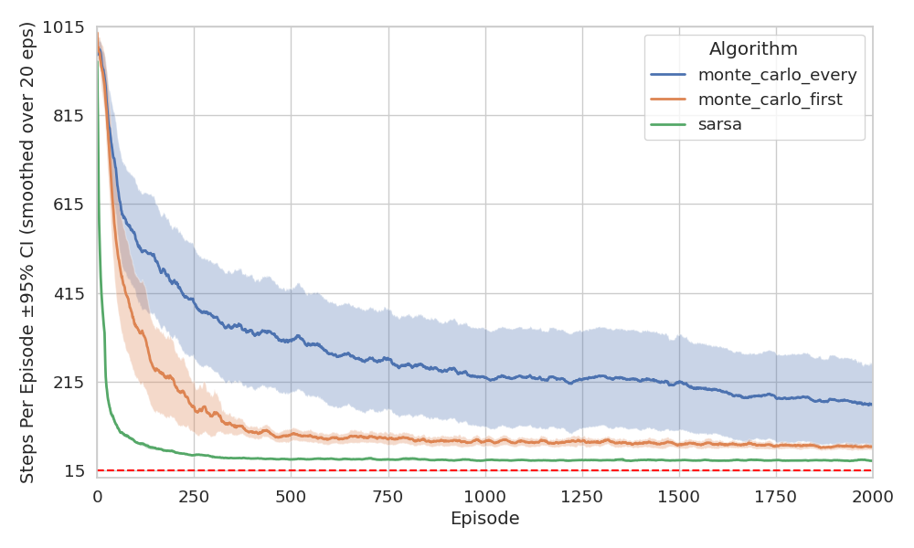
As expected, we see more uncertainty in the policies derived from MC methods. Although all methods eventually converge, TD converges faster in this environment. Unfortunately, we can’t currently back this claim with theory3, there’s still no formal proof that one method converges faster than the other. For now, it’s an open question.
learning rates analysis
In TD methods, the learning rate \(\alpha\) controls how much new information overrides prior estimates. A higher \(\alpha\) allows the agent to adapt quickly by placing more weight on recent rewards and bootstrapped values but can lead to instability. A lower \(\alpha\) yields more stable learning but slows down convergence.
In this section, we experiment with different constant learning rates,
within the ROOM_WITH_LAVA environment. Comparable results can also
be reproduced in the CLIFF environment.
For exploration, we use a soft \(\epsilon\)-greedy policy with \(\epsilon = 0.1\)
and \(\gamma = 1\) for all algorithms, varying \(\alpha\) over the small set of
\(\{0.001, 0.005, 0.01, 0.1\}\). Full configuration details are provided in
src/tasks/config/task2_1.yaml.
Figure 12 illustrates how the learned policies has converged under each setting:

The results align with theoretical expectations. As shown in Figure 12, smaller \(\alpha\) values lead to slower convergence, while larger \(\alpha\) values yield faster convergence for the Q-learning algorithm.
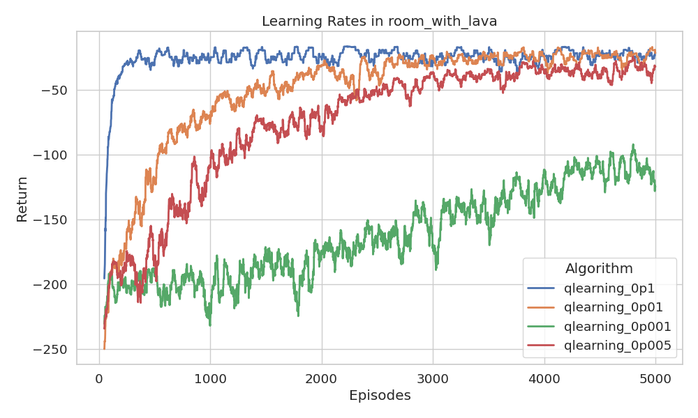
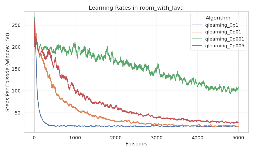
(smoothed with a window of episodes).
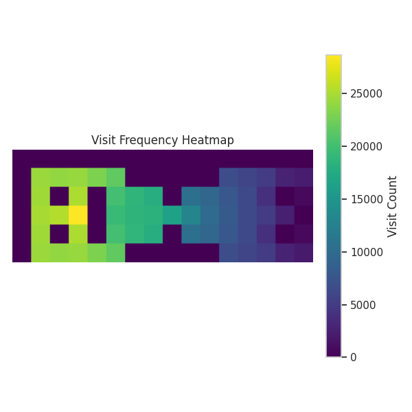
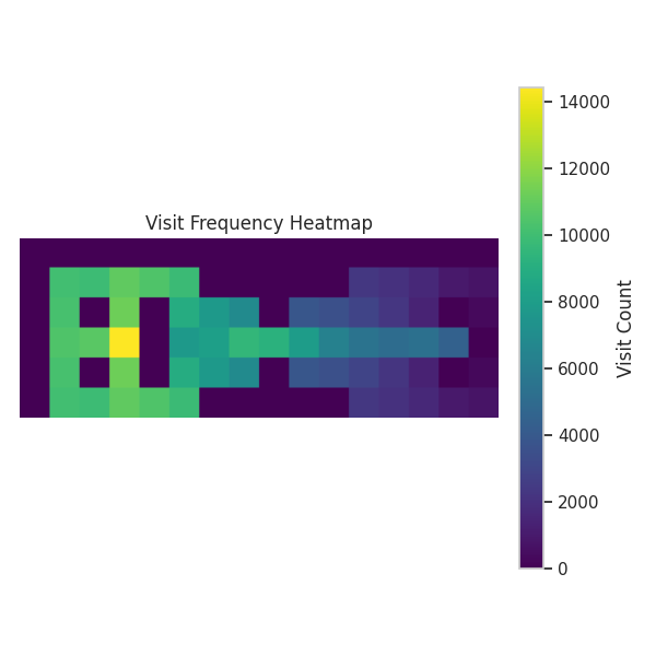
We also observe that the learning rate affects the agent’s exploration behavior. As shown in Figure 13, lower learning rates lead to broader exploration, while higher rates lead to more exploitative behavior. This aligns with theory3: a higher \(\alpha\) accelerates value propagation, which potentially stabilizes the policy sooner, leaving less time for exploration.
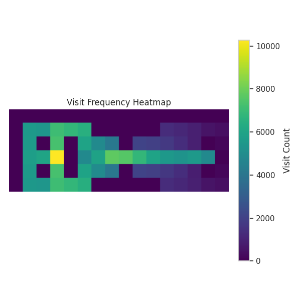
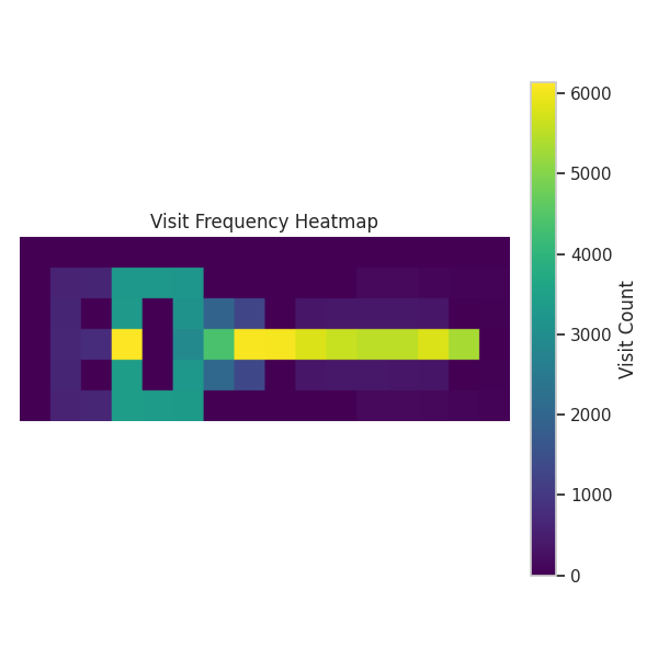
exploration-exploitation trade-off analysis
The \(\epsilon\)-greedy strategy selects a random action with probability \(\epsilon\), and follows the current policy otherwise. Setting \(\epsilon\) too high results in excessive randomness, preventing the agent from exploiting what it has learned. Conversely, making \(\epsilon\) too small limits exploration, possibly trapping the agent in suboptimal behaviors.
Here, we use a soft \(\epsilon\)-greedy policy with \(\epsilon \in
\{0.01,0.1,0.2,0.5\}\). The learning rate \(\alpha\) is fixed at \(0.1\)
and the discount factor \(\gamma\) is set to \(1\). Full configuration details
are provided in
src/tasks/config/task2_1.yaml.
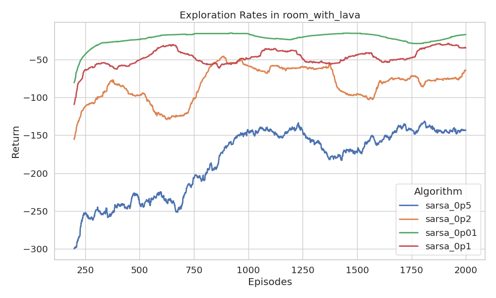
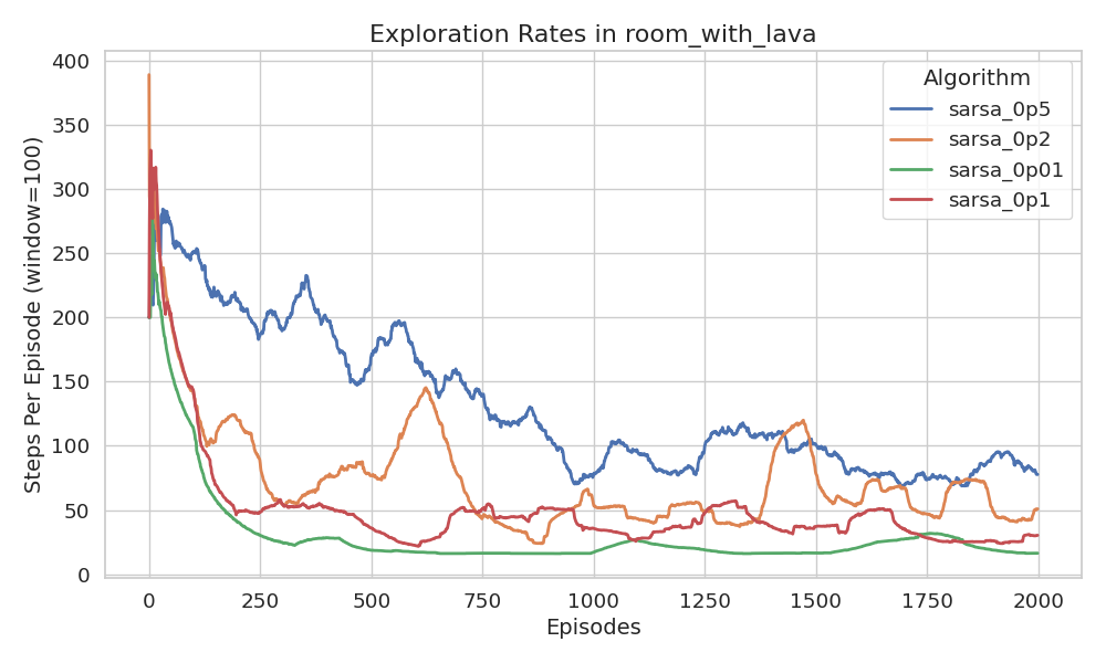
Surprisingly, the results show that almost zero exploration \((\epsilon = 0.01)\)
yields the highest return in the ROOM_WITH_LAVA environment. Similar outcomes
were observed in the CLIFF environment as well. At first glance, this seems
counterintuitive, but it makes sense given the characteristics of the environment.
Even though the environment allows for variance in the possible returns, the immediate reward for any given (state, action) pair is deterministic. There is no reward distribution to sample from. The agent always receives the same outcome for the same decision.
Additionally, as the agent explores, it accumulates \(-1\) penalties along each path, which inherently discourages revisiting those routes. This naturally drives the agent to favor unexplored (and potentially shorter or safer) alternatives, without needing random exploration.
In essence, the state space is small and simple enough that pure exploitation is sufficient to discover the optimal policy. The agent can locally maximize rewards and still converge to the correct solution, as verified by the empirical results. Interestingly, higher exploration rates degrade performance slightly, mostly due to increased chances of randomly stepping into lava. Nonetheless, all policies eventually converge.


2.2 Linear Exploration Rate
In the previous section, we experimented with different constant \(\epsilon\) values. Here, we instead use a linearly decreasing exploration schedule, where \(\epsilon\) progressively decays over the course of training. The goal is to start with broad exploration and gradually shift toward exploitation by reducing random action selection after each episode.
As noted earlier in the on-policy vs. off-policy section, both Sarsa and Q-learning converge to the same policy when \(\epsilon\) decreases over time. This section provides experimental evidence of that convergence.
We set the learning rate \(\alpha\) to \(0.1\) and use a linear decay
of \(\epsilon\) from \(0.01\) to \(0\) over 500 episodes. The discount
factor remains at \(\gamma = 1\). We evaluate the trained agent at
various checkpoints to observe the evolution of the target policy.
Full configuration details are available in
src/tasks/config/task2_2.yaml.

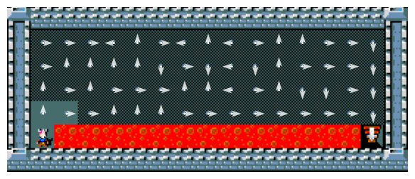
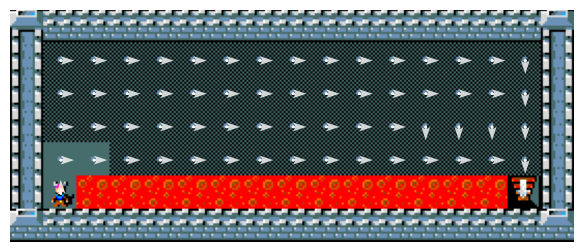
 After 50 episodes

 After 100 episodes

 After 200 episodes

 After 300 episodes

 After 400 episodes

 After 500 episodes
Each row corresponds to evaluations after some amount of episodes.
Note that Q-learning evaluates using a greedy policy, while Sarsa still follows an \(\epsilon\)-greedy policy during evaluation (unless \(\epsilon\) has decayed to 0).
From these experiments, we confirm that both Sarsa and Q-learning converge
to the same optimal policy when exploration is linearly decayed.
This confirms our theoretical expectations from earlier sections.
The complete implementation of the scheduling mechanism can be found in
the following file: src/schedule.py.
2.3 Planning and Learning
A model of the environment refers to any mechanism an agent can use to predict how the environment will respond to its actions. Given a state and an action, a model outputs the predicted next state and corresponding reward. The Dyna-Q implementation uses a table-based model under deterministic assumptions, when queried with previously seen state-action pairs, it simply returns the last observed next state and reward.
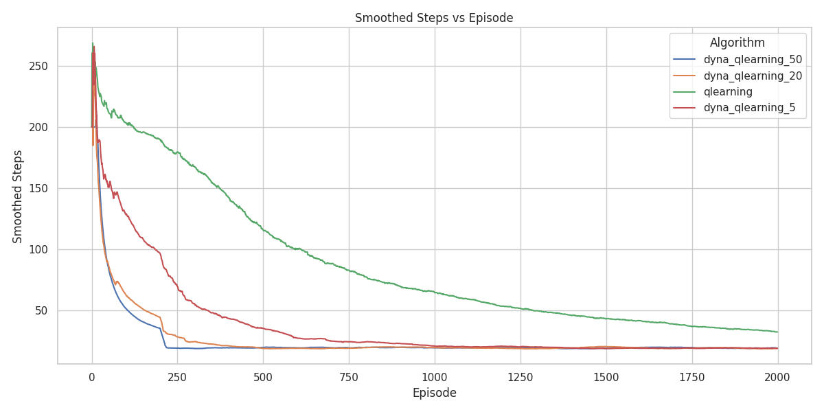
We will compare the performance of the Dyna-Q agent and the Q-learning
agent in two of the four Minihack environments. For exploration, we use a
soft epsilon-greedy policy with a constant \(\epsilon = 0.1\), \(\gamma = 1\)
and \(\alpha=0.01\). The number of planning steps is varied across \(\{0, 5, 20, 50\}\).
Full configuration details are available in
src/tasks/config/task2_3.yaml.


Even though all agents eventually reach optimal performance, Dyna-Q with 50 planning steps produces the cleanest, most symmetric policy. It correctly identifies that all paths that are functionally equivalent. Even with just 5 planning steps, Dyna-Q outperforms standard Q-learning by reducing unnecessary wall-directed actions in the outer regions.


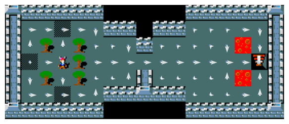
Figure 20 shows that planning agents converge faster than their non-planning counterparts. The agent with 50 planning steps has the fastest convergence. This is exactly what we expect. We expect that more planning would mean faster learning, where the agent with 50 steps would be the fastest.

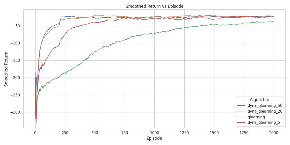
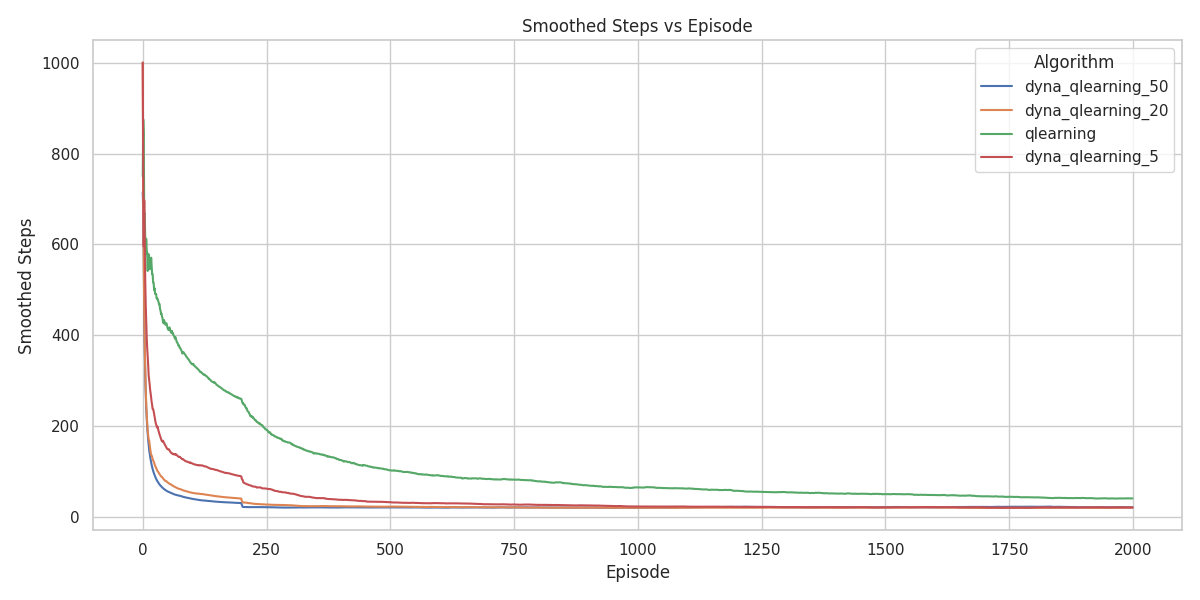
The superior performance of Dyna-Q in these tasks follows from the deterministic nature of the environments. If transitions and rewards are deterministic, then once the agent has experienced a state–action pair \((s,a)\) it can store the single observed next state and reward and use that stored tuple as a perfect model of the environment.
Each real interaction therefore yields not only one model-free Q-update but also many additional updates produced by repeatedly ‘imagining’ the same transition during planning. These extra updates accelerate value propagation and explain why agents with more planning steps converge faster in these deterministic settings.
This does not mean planning becomes useless in stochastic environments, it just means the sample model must also account for stochasticity. Instead of always returning the last observed next state and reward, the model should represent or sample from the observed variability so that planning reflects the true uncertainty in the environment.
3. Deep Reinforcement Learning
In this section, we implement deep reinforcement learning agents in
two environments: EMPTY_ROOM and ROOM_WITH_MULTIPLE_MONSTERS. The
second environment extends the first by introducing multiple randomly
spawning enemies, increasing the complexity and introducing stochasticity.
To handle this added challenge, we use two algorithms from the
stable_baselines3 library: DQN (Deep Q-Network), which applies
deep Q-learning, and PPO (Proximal Policy Optimization), which follows
the actor-critic framework. Despite transitioning to deep models, we
continue using an ASCII-based representation of the environment as the input state.
Since deep models require fixed-size input vectors, we convert the 2D ASCII map into a one-dimensional 64-dimensional embedding using a Convolutional Neural Network (CNN).
The CNN architecture consists of three convolutional layers with kernel
sizes of \((3,3)\), ReLU activations and padding to preserve spatial dimensions.
The output is then flattened and passed through a fully connected layer,
which outputs the 64-dimensional feature vector used as input to the
reinforcement learning algorithm. The implementation of this feature
extractor is available at
src/algorithms/cnn.py.
hyperparameter configuration
For training, we used a learning rate of 0.0001 for DQN and 0.0003 for PPO.
We used a discount factor \((\gamma)\) of 0.99 for both algorithms. For PPO,
we also added a small entropy bonus of 0.01 to encourage exploration. The
exact hyperparameters can be found in
src/tasks/config/task3_1.yaml.
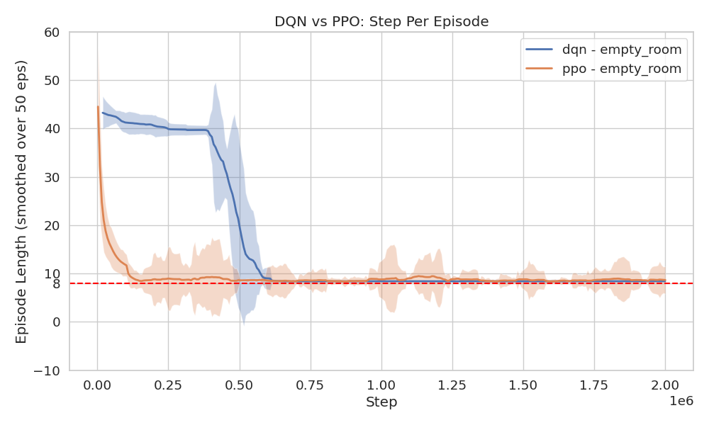
performance evaluation
Figure 21 shows that PPO trains
significantly faster and more stably than DQN. In the EMPTY_ROOM
environment, PPO converges in roughly 250 000 steps, while
DQN requires nearly 750 000!
The number of training steps required can partly be attributed to the high-dimensional state representation processed by the CNN. If a more compact, handcrafted representation were used instead, a simpler model with fewer parameters could possibly converge much faster.
The gap is even more pronounced in the ROOM_WITH_MULTIPLE_MONSTERS
environment, PPO still converges within 250 000 steps, but DQN needs
nearly 2 million steps.
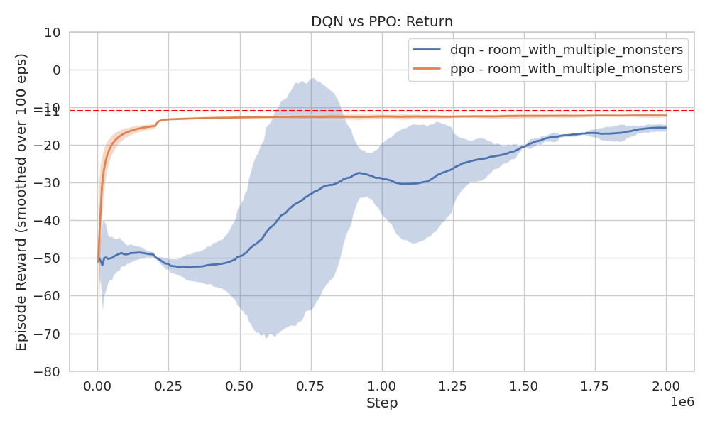
Despite both DQN and PPO eventually learning near-optimal policies, behavior differs: DQN only eliminated the monster closest to the start position and then heads straight to the goal, avoiding other enemies. PPO, in contrast, clears out all monsters along the way before proceeding to the goal.
Figure 22 illustrates full episodes in both environments for each agent.


Tabular-Q vs DQN
-
Convergence Speed: Tabular methods converge much faster due to the limited, discrete state space in grid-based environments. They typically require only hundreds of thousands of steps, while DRL methods possibly need millions.
-
Generalization: Tabular Q-learning memorizes state-action pairs and lacks generalization. It fails on slightly altered environments (e.g., grid size changes). In contrast, DRL models (especially CNN-based ones) can generalize better across similar but unseen states. For instance, a model trained on a \(5 \times 5\) grid might still operate reasonably on a \(6 \times 6\) one, something tabular Q cannot do.
-
Convergence Guarantees: Under certain assumptions, tabular methods guarantee convergence to the optimal policy. DRL methods do not, they may converge to suboptimal or unstable policies depending on architecture, hyperparameters and randomness.